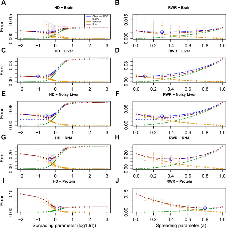
Fig 2. Bias-variance decomposition of the Mean Squared Error (MSE).

Mean squared error curve (blue, averaged across samples) across the values of the spreading parameter for the brain (A, B) and liver (C, D) and for the liver data with added noise (E, F) in Ori et al. [13] dataset, and for the mRNA (G, H) and protein layer (I, J) in the PCa dataset using HD (A, C, E, G, I) and RWR (B, D, F, H, J). Minimum MSEs are circled (blue). Additionally, the decomposition is depicted: the bias² curve (green), the variance curve (orange) (as defined in Material and Methods) and their sum (red) are shown. The sum (red curve) approximates very well the observed MSE (blue curve). For the quantities with replicate values (i.e. observed MSE, variance and sum), error bars have been added to represent the actual distribution at the respective spreading parameters. The replicate data is firstly log-transformed. Subsequently, the average and standard deviation (SD) across the six replicates is computed for each value of the spreading parameter in the transformed space. Finally, the average, the lower error bound (average-SD) and the upper error bound (average+SD) in the log-transformed space are transformed back to the original space (i.e. the points correspond to the geometric mean). In (E, F), the dashed curve (blue) corresponds to the MSE curve of the original liver data (i.e. the (blue) curve depicted in (C) and (D) respectively).