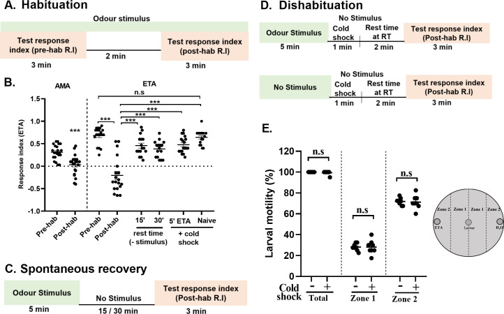
Fig 1. Olfactory habituation assay in wild-type Drosophila larvae.
(A) Schematics represent the specific time segments to induce olfactory habituation in wild-type (W1118) larvae. Naïve larvae were exposed to the odour and response index (R.I) was calculated after 3 min (Pre-hab R.I). The same set of larvae were left for additional 2 min in presence of odour for habituation (This makes total odour exposure time to 5 min). The odour exposed larvae were brought back in the middle of the petriplate and the R.I was again calculated (Post-hab R.I). (B) Scatter plot shows response indices (R.I, black circles) of naïve wild type larvae towards amyl acetate (AMA) or ethyl acetate (ETA) (pre-hab R.I) and after 5 min of odour exposure (post-hab R.I). Larvae pre-exposed to odour for 5 min shows spontaneous recovery after 15 or 30 min in the absence of stimulus (see spontaneous recovery schematics). Larvae pre-exposed to odour for 5 min shows recovery by 1min cold shock (5’ETA+cold shock), the phenomenon called dishabituation (see dishabituation schematics). R.I of naïve larvae without odour pre-exposure but exposed to cold shock (Naïve+cold shock) is not altered due to cold shock. (C) Schematics represent the specific time segments to induce spontaneous recovery, (D) Schematics represent the specific time segments to induce dishabituation. (E) The scatter plot shows percent larval motility of 1 min cold shock treated (+) and untreated larvae (-), in a petriplate with ETA and water on opposite ends. As shown in the schematics on right, the larvae were kept in the centre and after 3 min, the total number of larvae that moved to different zones were counted. The data represented here shows percentage of total larvae moved, larvae moved to zone1, and zone 2, N = 8. Data is represented as scatter plot with error bars showing SEM and N≥16, unless mentioned. Each N represent one experiment performed with a group of 30–40 larvae. Each data group was analysed for normal distribution using Shapiro-Wilk test. Statistical significance was determined by two-tailed unpaired t-test (parametric) with Welchs correction. *** represent p≤0.0001, n.s means statistical non-significance when p≥0.05. For statistical details and numerical data values in the scatter plot refer to S1 and S2 Data.

