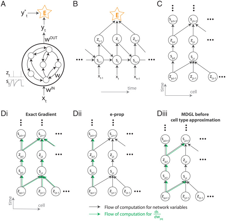
Fig. 6.

Computational graph and gradient propagation. (A) Schematic illustration of the recurrent neural network used in this study. (B) The mathematical dependencies of input x, state s, neuron spikes z, and loss function E unwrapped across time. (C) The dependencies of state s and neuron spikes z unwrapped across time and cells. (D) The computational flow of $\text{d}s/\text{d}{w}_{pq}$ is illustrated for exact gradients computed using exact calculation (Eq. 17) (i), e-prop (ii), and our truncation in Eq. 18, where dependency within one connection step has been captured (iii). Black arrows denote the computational flow of network states, output, and the loss; for instance, the forward arrows from z_t and s_t going to $s_{t+1}$ are due to the neuronal dynamics equation in Eq. 2. Green arrows denote the computational flow of $\text{d}s/\text{d}{w}_{pq}$ for various learning rules.