Figure 4. Displacement detector (DD) model of small object motion detection.

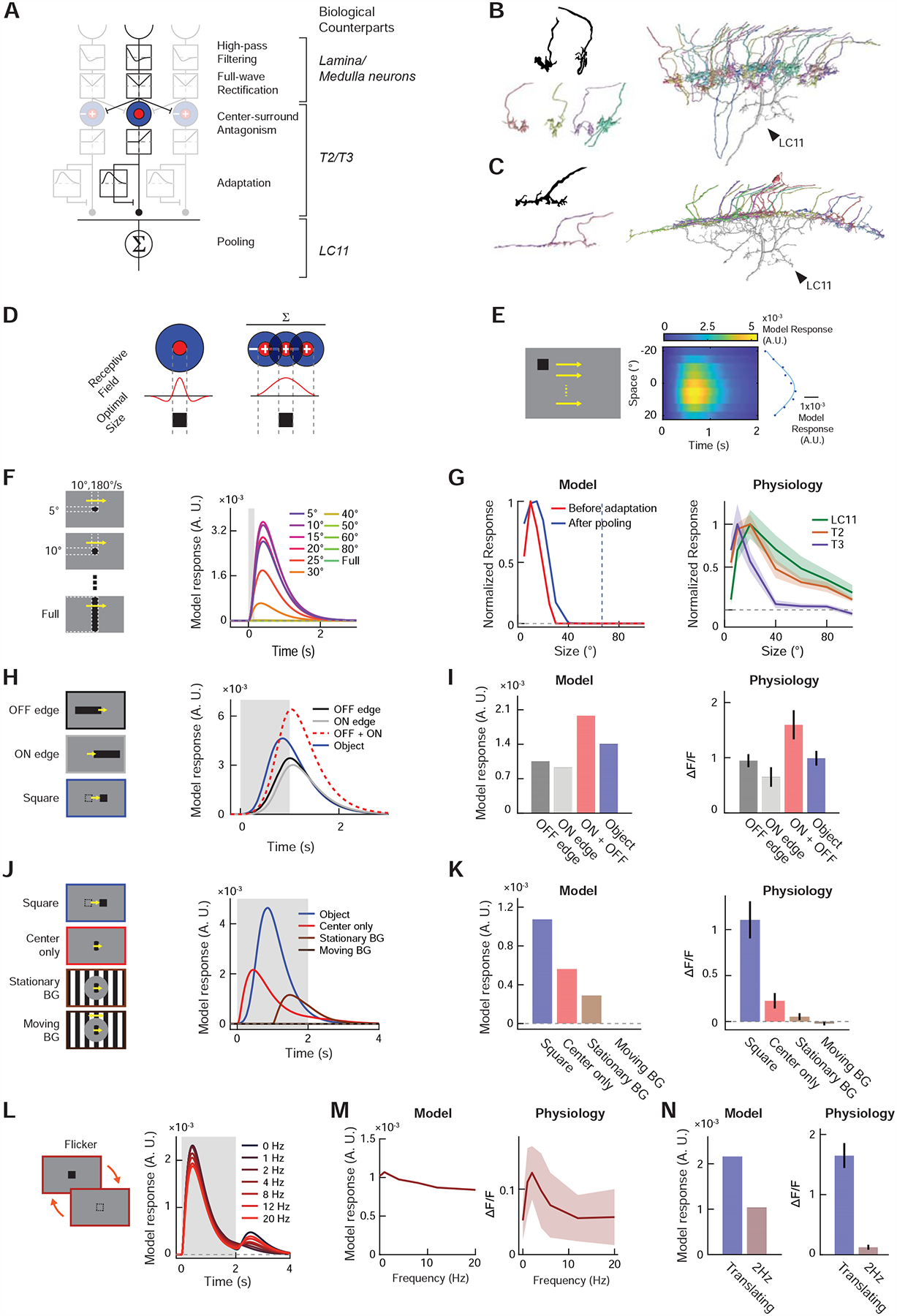
(A) The DD model consists of initial temporal high-pass filtering and full-wave rectification, center-surround antagonism, adaptation by divisive inhibition, and spatial pooling (see STAR Methods). Putative neuronal bases of each algorithmic step are indicated in italic. (B) (top left) Golgi-staining based camera lucida drawing of T3 terminals, from [22]. (bottom left) Putative T3 terminals found among presynaptic neurons of the particular LC11 neuron shown in Figure S7B. (right) The 33 putative T3 terminals we identified among the presynaptic cells of the LC11 shown in Figure S7B. See Table S1 for their unique identifiers in the hemibrain dataset. T3 appears to tile the entire dendritic arbor of LC11 in Lo2/3, supporting the proposed pooling motif in the DD model. (C) (top left) Golgi-staining based drawing of a T2 terminal, from [22]. (bottom left) Putative T2 terminals found among presynaptic neurons of the same LC11 neuron. See Table S1 for their unique identifiers in the hemibrain dataset. (right) The 23 putative T2 cells identified among presynaptic partners of the LC11 neuron. Similar to T3, T2 also appears to tile the entirety of the LC11 dendrite in Lo2/3. (D) In a neuron where center-surround antagonism establishes its size tuning, the size of excitatory receptive field and its optimal object size must be equal. Neurons that pool already size-tuned inputs can have larger receptive field sizes than the optimal object size. (E) Model responses (right) to horizontally translating squares (left) used for RF mapping in Figure 3C. Blue dots indicate time-averaged responses by each elevation, and the blue curve a Gaussian function fitted to the dots. (F) Model responses to objects with various sizes, as in Figure 3E. (G) (left) Size-tuning curves of the output unit (red) and input unit before adaptation (blue). The blue dotted line indicates the RF size, calculated as the FWQM value of the Gaussian function in (E). (right) Physiologically measured size-tuning curves of LC11 and its putative inputs, T2 and T3, replotted from Figures 3F, S6F, S5G, respectively. (H) Model responses to decoupled edge stimuli, along with simulated sum of its responses to ON and OFF edges, as in Figure 3H. (I) Time-averaged model responses to decoupled edge stimuli (left), along with corresponding physiological results (right), replotted from Figure 3I. (J) Model responses to localized gratings with or without stimuli in the background and a translating square, as in Figure 3K. (K) Time-averaged model responses to localized grating stimuli (left), along with corresponding physiological results (right), replotted from Figure 3L. (L) Model responses to stationary squares that flickered at different temporal frequencies, as in Figure 3M. (M) Temporal frequency tuning curve of the model (left) and LC11 cells (right). The latter was replotted from Figure 3N. (N) Comparison of model (left) and physiological responses (right) to either translating or flickering square at 2Hz. The latter was replotted from Figure 3O.