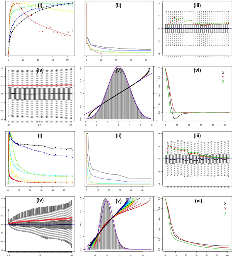
Fig. 2.

Diagnostics associated with the Image-Domain Bootstrapping Model (2). Rows 1&2 correspond to the FDG-Brain data; Rows 3&4 to the FLT-Breast data. Six plots, labeled (i) to (vi), are shown for each dataset: (i) raw sub-TACs (dots) and fitted models (lines) for the selected basis set - columns of X. (ii) Non-parametric residues corresponding to the fitted model - c.f. (10). (iii) Boxplots by time-frame of standardized residuals from the unconstrained least squares fit, $r_{ij}∕{\widehat{\sigma }}_i{\widehat{\varphi }}_j{\widehat{h}}_{ij}$. The simple, ${\widehat{\varphi }}_j^0$ in (5), and optimized, ${\widehat{\varphi }}_j$, standard deviations are shown as green and red dots. (iv) Boxplots of scaled residuals, ${\widehat{ϵ}}_{ij}=r_{ij}∕{\widehat{\sigma }}_i{\widehat{\varphi }}_j$, for each κ-bin (each containing roughly 10,000 data points). ${\widehat{h}}_l$-values are shown as red points; the red line is for comparison with unity (zero skewness of bin data). (v) Histogram of the overall distribution of the standardized residuals and its relation to a Gaussian fit (purple curve). Super-imposed are points showing quantiles of standardized residuals from different κ-bins (colored from red to dark blue according to bin order) versus corresponding quantiles of the Gaussian (right y-axis). The quantile pattern for the overall histogram and the Gaussian fit are shown with dashed black and purple lines. (vi) Directional auto-correlation patterns of the normalized residuals, $\widehat{\eta }$ (see section 2.4), as a function of distance in millimeters. X-Y are transverse with Y perpendicular to the scanning bed; Z is the axial direction.