FIGURE 3.

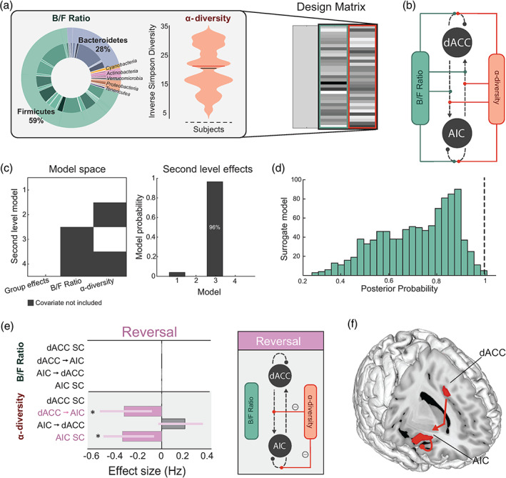
Effects of high‐level microbial properties on threat learning and updating. (a) Inlet (left) shows the mean proportions of B/F, and the violin plot (middle) shows the distribution of α‐diversity (Inverse Simpson diversity) scores in our samples (n = 38). These two microbiota features constituted our two regressors in the Parametric Empirical Bayes model (design matrix columns two and three, right). The first column models the group mean. (b) Specification of the model space showing all possible modulatory connections where the microbiota features can interact within the AIC‐dACC network. (c) Model space (left) showing possible second level models (including a null model), where both covariates (Model 1), one covariate (Models 2 and 3), or no covariates (Model 4, null) contribute to the model evidence. The winning second level model (right) included the second covariate (Model 3), at a posterior probability (Pp) of 0.96. (d) Distribution of Pp results from surrogate testing. Dashed black line indicates the Pp (0.96) of the winning model for the original (nonpermuted) data. (e) Results from Bayesian Model Reduction (BMR) showing the effect sizes (expressed in Hz) of modulatory connections associated with α‐diversity during threat reversal. Significant parameters are those with a Pp > 0.95, indicated with an asterisk. The length of the bars corresponds to the expected probability (Ep) and the error bars are 90% Bayesian confidence intervals. SC represents self‐connections. (f) Anatomical representation showing the significant modulatory connections associated with α‐diversity during the threat reversal phase