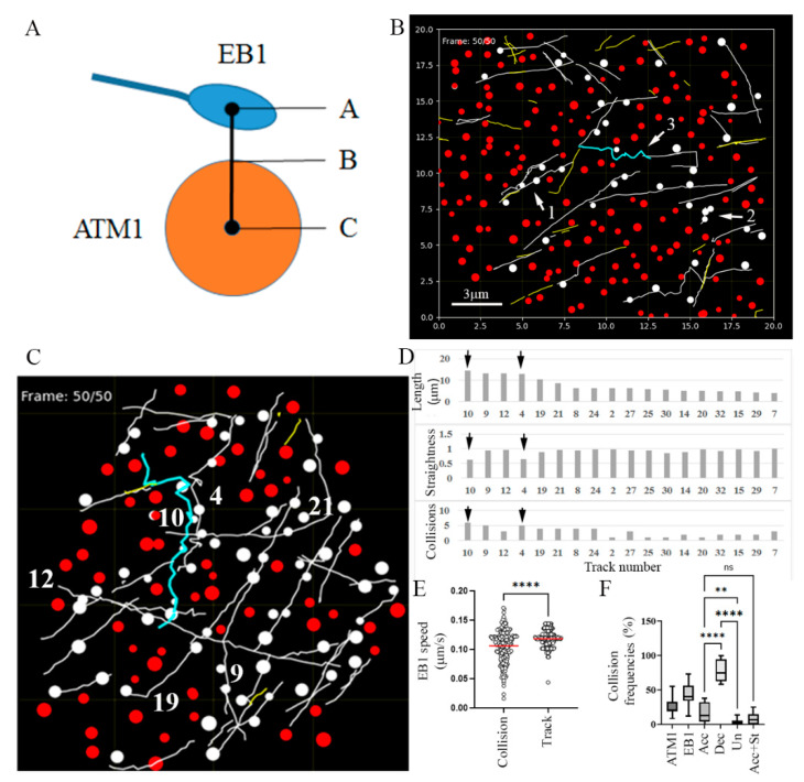
Figure 5.

A software program developed in Python that simulates MTs–ATM1^IQ-tail collisions. (A) Scheme showing the concept of the simulation: coordinates of the positioning of each ATM1^IQ-tail cluster or EB1b spot were extracted from Imaris. A collision was counted when the distance from A to B was ≤100 nm. (B) Snapshot of animation based on Movie S5. Spots of ATM1^IQ-tail that experience MTs collision and the colliding track turned white. A selected track was colored. Arrows indicate three of the four scenarios: (1) pass through, (2) pause and disappear, (3) wave and change direction. Scale bar = 3 μm. (C–E) A comparison of all tracks by a single cell analysis. (C) Snapshot of the last frame of the animation (Movies S8 and S9) showing, in white, tracks and spots that experienced collisions. The numbers show the six longest tracks. Track 10 which experienced maximum collisions is colored. (D) Summary of length, straightness and number of collisions for all tracks above 5 μm in length. Arrows show tracks 10 and 4 as being the least straight. (E) EB1b speed in frames −1 to +3 around every collision compared to the average speed along the whole track. The graph shows results from the cell presented in panel (C). Differences were determined by t-test p < 0.0001. (F) Collisions frequencies calculated in 20 cells; ATM1-percent ATM1^IQ-tail spots experienced collisions, EB1-percent colliding tracks, Acc-percent tracks with accelerated speed after a collision. Dec-percent tracks with decelerated speed after a collision. Un-percent tracks with unaffected speed. Acc + str-percent tracks with accelerated speed associated with decreased straightness. ** p < 0.01, **** p < 0.0001 one way ANOVA. ns = not significant.