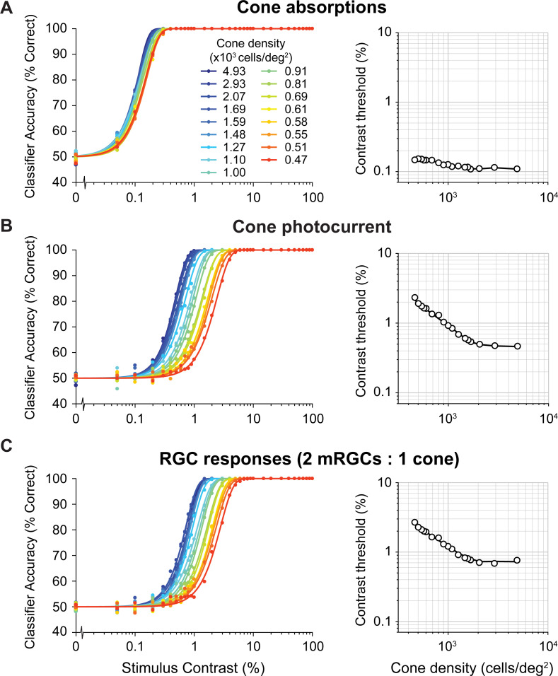
Fig 5. Model performance for different computational stages.

Left column shows classifier accuracy as function of stimulus contrast. Data are from simulated experiments with 1,000 trials per stimulus class, using a model with a L-cone only mosaic varying in cone density. Data are fitted with a Weibull function. Contrast thresholds are plotted separately as a function of cone density in the right column. (A) Cone absorptions. Applying a linear SVM classifier to cone absorptions averaged across stimulus time points. (B) Cone photocurrent. Applying a linear SVM classifier to cone outer segment photocurrent responses, averaged across time weighted by a temporally delayed stimulus time course. This transformation of cone absorptions into photocurrent causes a ~10x increase in contrast thresholds, interacting with cone density (i.e., Weibull functions are spaced out compared to cone absorptions). (C) RGC responses. Applying a linear SVM classifier to spatially filtered photocurrent with added white noise. This transformation causes an additional increase in contrast thresholds for all cone densities. Data show results for a fixed subsampling ratio of 2 mRGCs per cone.