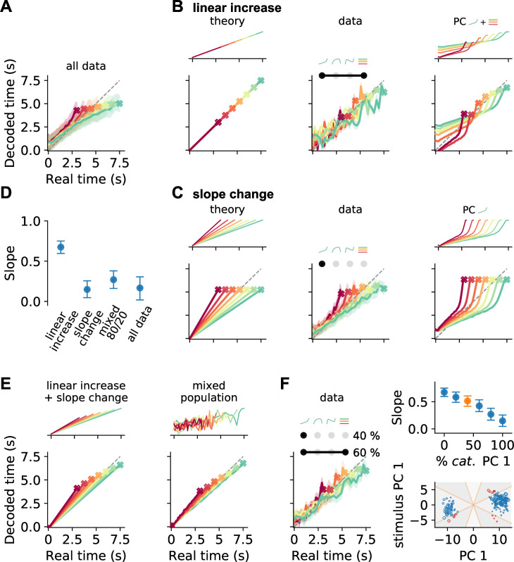
Figure 7. Decoding elapsed time from prefrontal population activity.

(A) Elapsed time (average ± standard deviation from bootstrapping) decoded from the responses of all neurons recorded during the reproduction phase. As before, color identifies stimulus duration. Crosses mark final values. A strong regression effect is visible. (B) Time decoding with neurons that ramp to stimulus-dependent levels but with the same slope and (C) with ramp-to-threshold cells. Left panels illustrate the theoretical prediction for decoded time and example neuronal activity above. Middle panels plot decoding results using only neurons from the respective response category. Right panels give results for decoding using the corresponding components from demixed principal component analysis (PCA). As displayed in the top panels, these components are principal component (PC) 1 and stimulus PC 1 in (B); and PC 1 only in (C). (D) Median slopes of the linear regression between the final values of real and predicted time for decoding from data in (A–C) and for a mixture of 80% slope-changing and 20% linear increasing cells, which aligns well with decoding from all data (A); regarding mixtures see also (F). Error bars delimit interquartile ranges (from bootstrapping). (E) Mixtures of linear increasing activity and slope changes explain behavioral regression effects. Theoretical predictions for mixing both responses in single neurons (left) or as two different response types across a population (right). For the second case, a neuron with noisy linear increasing activity is displayed as an example. (F) Decoding results for a mixed population of 40% slope-changing and 60% linear increasing cells. The cells were sampled at these fractions in each bootstrapping run from the response categories we identified in our recorded data. The upper-right panel shows the regression slope (D) for different fractions of slope-changing cells. The orange marker corresponds to the example in the left panel. The lower-right panel displays the PCA scores of the cells from the linear increasing (red; PC 1 + stimulus PC 1) and slope-changing categories (blue; PC 1 only). The size of the marker illustrates the decoder weight $\beta$ for that cell. See also Figure 5—figure supplement 4C.

Figure 7—figure supplement 1. Decoding elapsed time from data, shuffled data, and noise.

Decoding results from the whole population, cells with sufficiently large dPCA scores, cells with small dPCA scores (‘unrelated activity’), shuffled data and noise during the reproduction phase. Each panel displays decoded time vs. the real time for each stimulus (color coded); average ± standard deviation (from bootstrapping). Crosses mark final values. Number of neurons is given in the lower-right corner. Rightmost panels display slopes and indifference points of linear regression between final values of real and predicted time for the five data sets. At the indifference point, real and decoded final time match. We calculated it from the slope and intercept of the regression line as $\frac{\text{intercept}}{1-\text{slope}}$. The indifference point estimates the amount of general over-/underestimation. With a regression effect, the indifference point should be at the center of the stimulus distribution (5.25 s), which we only obtain when decoding from all data or the cells with large principal component analysis (PCA) scores.

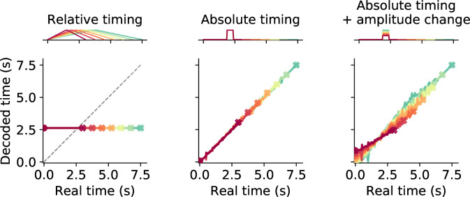
Figure 7—figure supplement 2. Decoding time from phasically active neurons.

Decoding results for three different theoretical response types with phasic activation. The uppermost panel in each column shows example neuronal activity and the panel below gives the prediction for decoded time. Different stimulus intervals are color coded. Crosses mark final values. Relative timing neurons peak at the center of an interval. Absolute timing neurons peak at a specific time point. In addition, stimulus interval may be coded in the response amplitude (absolute timing + amplitude change). Although only one example is displayed, for both types of absolute timing neurons the population comprises cells peaking at different time points such that the whole interval is tiled. Relative timing neurons can only encode a single time point, whereas absolute timing neurons allow for precise time encoding.

Figure 7—figure supplement 3. Decoding time during measurement.

Results are displayed for all data (left), cells in the principal component (PC) 1 + stimulus PC 1 category, and cells in the PC 1-only category. For all data, decoding is imprecise with initial overestimation and underestimation at the end of the interval. For PC 1 + stimulus PC 1 cells as well as cells in the PC 1-only category, decoded time starts out more precisely but ends up at a general underestimation for the first response type. However, a regression effect with an overestimation for small stimuli is visible in the second case.