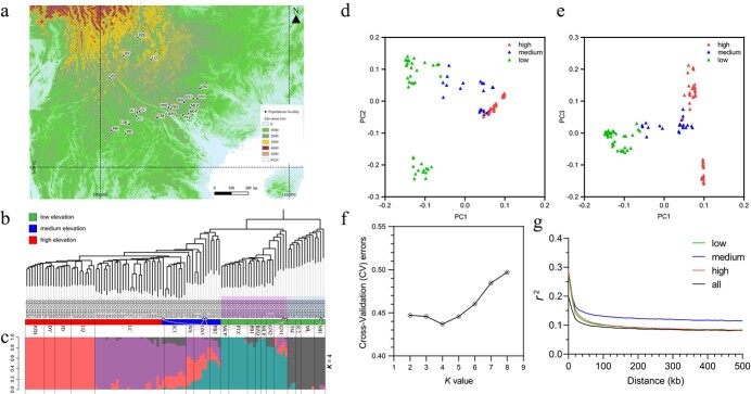
Figure 2.

Ilex polyneura population localities sampled in this study and population genetic analyses. a, Localities of sampled populations projected on an elevation map based on SMRT data with 30 arc-second resolution (https://www.usgs.gov/centers/eros/science/usgs-eros-archive-digital-elevation-shuttle-radar-topography-mission-srtm-1-arc?qt-science_center_objects=0#qt-science_center_objects) using QGIS software v.3.6.3 (http://www.qgis.org). b, Phylogenetic analysis of the 112 individuals with the neighbor-joining (NJ) method using the filtered SNPs. Green, blue, and red strips next to the individual names indicate low, medium, and high elevations. Populations are labeled by their names. Six individuals who were not clustered with other individuals in the same population are labeled with black empty circles and linked with their home populations by pink lines. c, Population genetic structure with the best K value (K = 4). d and e, PCA of genetic variation in the 21 populations. f, Cross-validation error rate of different K values from the population genetic structure analysis. g, Analysis of linkage disequilibrium (LD) decay in the 21 populations, in which the y-axis indicates that the linkage disequilibrium decays with genomic pairwise distance (x-axis) in low elevation populations (green line), medium elevation populations (blue line), high elevation populations (red line), and all populations (black line).