Figure 5. ORN-valence combinations follow complex rules.

(A) Valence responses of the single-ORN lines used to generate ORN-combos (replotted from Figure 1). The dots represent the mean valence between control (N≅ 104) and test (N ≅ 52) flies (∆wTSALE with 95% CIs). The shades of red signify the three light intensities. (B) The valence responses produced by the ORN-combos in the WALISAR assay in three light intensities. (C–E) ORN-combo valences as predicted by the summation (C), max pooling (D) and min pooling (E) models. (F) Three positive (green), two negative (magenta), and three neutral (gray) ORNs were used to generate seven ORN two-way combinations. (G–I) Scatter plots representing the influence of individual ORNs on the respective ORN-combo valence. The red (G), maroon (H), and black (I) dots indicate ORN-combos at 14, 42, and 70 μW/mm² light intensities, respectively. The horizontal (β₁) and vertical (β₂) axes show the median weights of ORN components in the resulting combination valence. (J) Euclidean distances of the ORN-combo β points from the diagonal (summation) line in panel J. The average distance increases as the light stimulus intensifies: 0.14 [95CI 0.06, 0.23], 0.20 [95CI 0.06, 0.34], and 0.37 [95CI 0.20, 0.53], respectively. (K) The β weights of the ORN-combos from the multiple linear regression are drawn as the signed distances of each ORN-combo from the diagonal line over three light intensities. The ORN weightings change magnitude and, in a few cases, the dominant partner changes with increasing optogenetic stimulus.

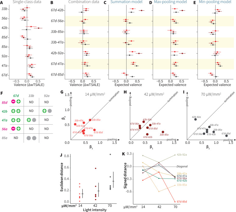
Figure 5—figure supplement 1. Linear analyses of combination valence results.

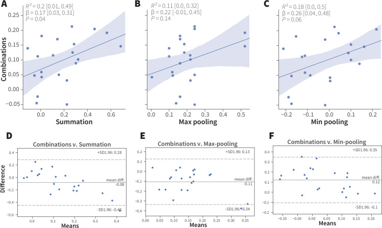
(A-C) Simple linear regression analyses of the experimental ORN-combo results and the predictions by the (A) summation, R2 = 0.2 [95CI 0.01, 0.49], p = 0.04; (B) max-pooling R2 = 0.11 [95CI 0.00, 0.32], p = 0.14; and (C) min-pooling R2 = 0.18 [95CI 0.0, 0.5], p = 0.06 functions. (D–F) Agreement analysis of the observed and predicted ORN-combo valence responses by three pooling functions. Bland-Altman plots of ORN-combo valence responses and predictions by the (D) summation, (E) max-pooling, and (F) min-pooling models. Even though the mean difference of the two tested values (y axis) is low in all models, the limits of agreement (SD –1.96, + 1.96) are sufficiently wide for them to be considered dissimilar.

Figure 5—figure supplement 2. Bootstrapped distributions of β weights of the ORN-combo constituents.

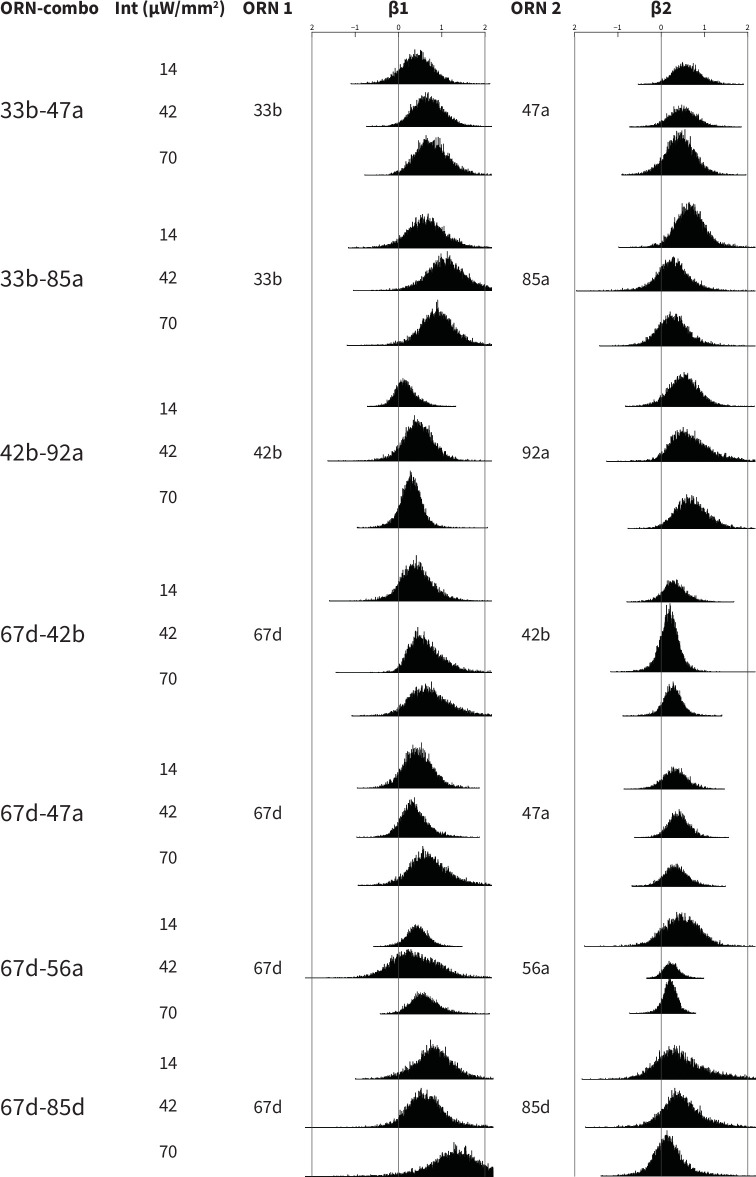
Associations between ORN-combos and their constituent single-ORN types are tested by using a multiple linear regression analysis approach. ORN1 and ORN2 columns indicate the odor receptor types that are used to generate the respective ORN-combo. The light intensity used in the experiments are shown in the intensity (Int; µW/mm²) column. β1 and β2 columns present the bootstrapped β distributions of the ORN1 and ORN2, respectively; the y axes indicate the count, and are all plotted using the same scale.

Figure 5—figure supplement 3. A linear model accounts for only 23% of the variance in odor behavior.

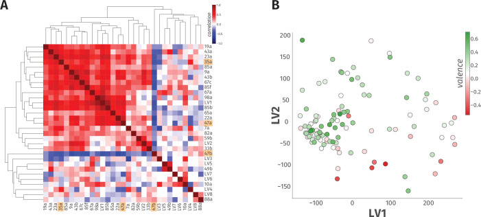
(A) The heatmap of hierarchical clustering shows the 27 × 27 Pearson correlation coefficients among the 23 ORN types and eight LVs from PLS-DA analysis. The internal correlation of LVs and their constituent ORN-types is indicated by color, where blue and red ends of the spectrum represent negative and positive correlations, respectively. The three ORN types that produced a valence response in the WALISAR screen are highlighted in orange. (B) A scatter plot displays projection of 110 odorants to two-dimensional LV space. The valence of the odorants are shown with a color gradient ranging from red to green, indicating aversive and attractive odorants, respectively.

Figure 5—figure supplement 4. Non-linear models suffer from the small size of the odor-valence data set.

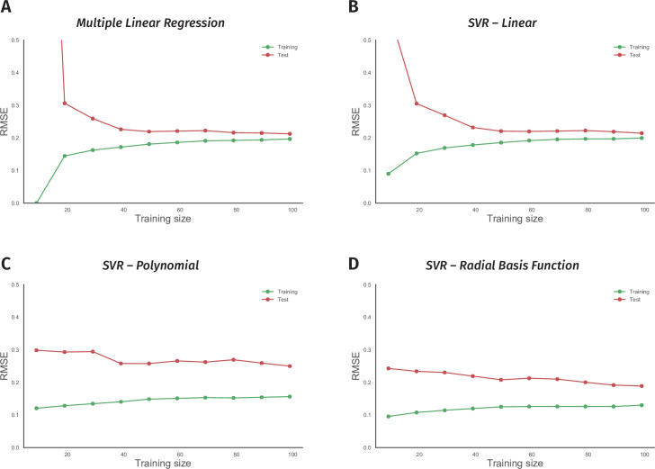
(A) Performance of a multiple linear regression (MLR) model is shown as the training data size is incrementally increased. The y-axis indicates the root-mean-squared-error (RMSE), while the x-axis is the size of the training data-set. The green and red traces in all the panels represent error rates on training and 10-fold cross-validation test data, respectively. (B) Learning curve of a support vector regression (SVR) model with a linear kernel is drawn. Both MLR and SVR linear models show convergent learning curves. (C) Performance of a support vector regression (SVR) model using a non-linear, polynomial kernel is plotted over an increasing training data-set size. (D) Error rates of a support vector regression (SVR) model with a non-linear, radial-basis-function kernel are plotted over a growing training data size. Both nonlinear models’ learning curves fail to converge, indicating overfit.