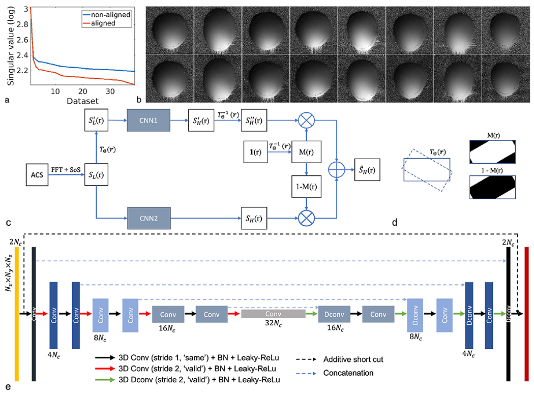
Figure 1.

Main assumption and idea of DeepSENSE. a) Singular values of the Casorati matrix formed by stacking all the 3D sensitivity maps as its columns, demonstrating the low-dimensionality of the 3D coil sensitivity from the head coil. The 3D sensitivity maps are derived from the GRE dataset obtained from 15 subjects in this study. b) Example 2D sensitivity maps (i.e., same coil and same slice index) of each 3D volumes from eight different subjects before (top row) and after (bottom row) sensitivity alignment w.r.t. the first scan. With proper alignment, intensity variation in the sensitivity maps towards those in the first scan can be observed, leading to a lower-dimensional representation in the linear subspace. c) Workflow of the proposed method for improved sensitivity estimation from limited ACS data using deep learning; d) Illustration of spatial masks M (r) and 1 − M (r) to combine the predictions from the two CNNs in the case of a clockwise rotation. The mask M (r), calculated using 1 ($T_{\text{Θ}}^{-1}(\mathbf{r})$), indicates signals remaining in the FOV (intersected area between solid and dashed rectangles) that can be selected from the prediction of CNN1 while 1 − M (r), the area around the corner, corresponds to signals transformed out of the FOV, which can only be predicted from CNN2. e) The structure of the convolutional neural network used in the proposed method. The first orange and last red layers represent the input and output 3D sensitivity functions respectively. The intermediate layers are color coded differently at different scales. The number of feature maps is listed on the top or at the bottom of the corresponding layer. Layers from the same scale have the same size of feature maps. N_x × N_y × N_z and N_c denote the spatial dimension in 3D and the number of head coil channels respectively.