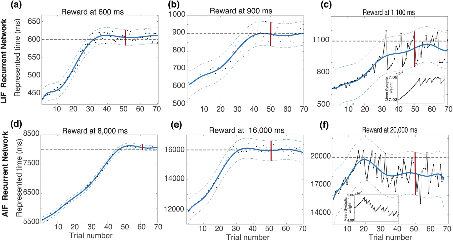
Figure 5:

Learning reward times using RDE in recurrent networks with and without active conductances. Network decay time (T) changes are plotted with respect to training trials for different target times and for both LIF (top plots) and AIF (bottom plots) models. Learning reward times with LIF model (top). For 600ms, and 900ms (a and b) learning is stable, but for 1100ms (c), the learning leads to large fluctuations. Inset shows weight fluctuations which lead to large decay time fluctuations. Learning reward time AIF model (bottom). For 8,000ms, and 16,000ms (d and e) but for 20000ms (f), learning leads to large fluctuations. In all plots, thick dashed gray lines show target decay times, filled circles decay time on single trial, blue line is a moving average, thin dashed lines confidence interval of the decay times, and vertical red bar is the confidence interval used for determining if learning is stable