Extended Figure 10. Computational model of neural folding recapitulates in vitro morphology.

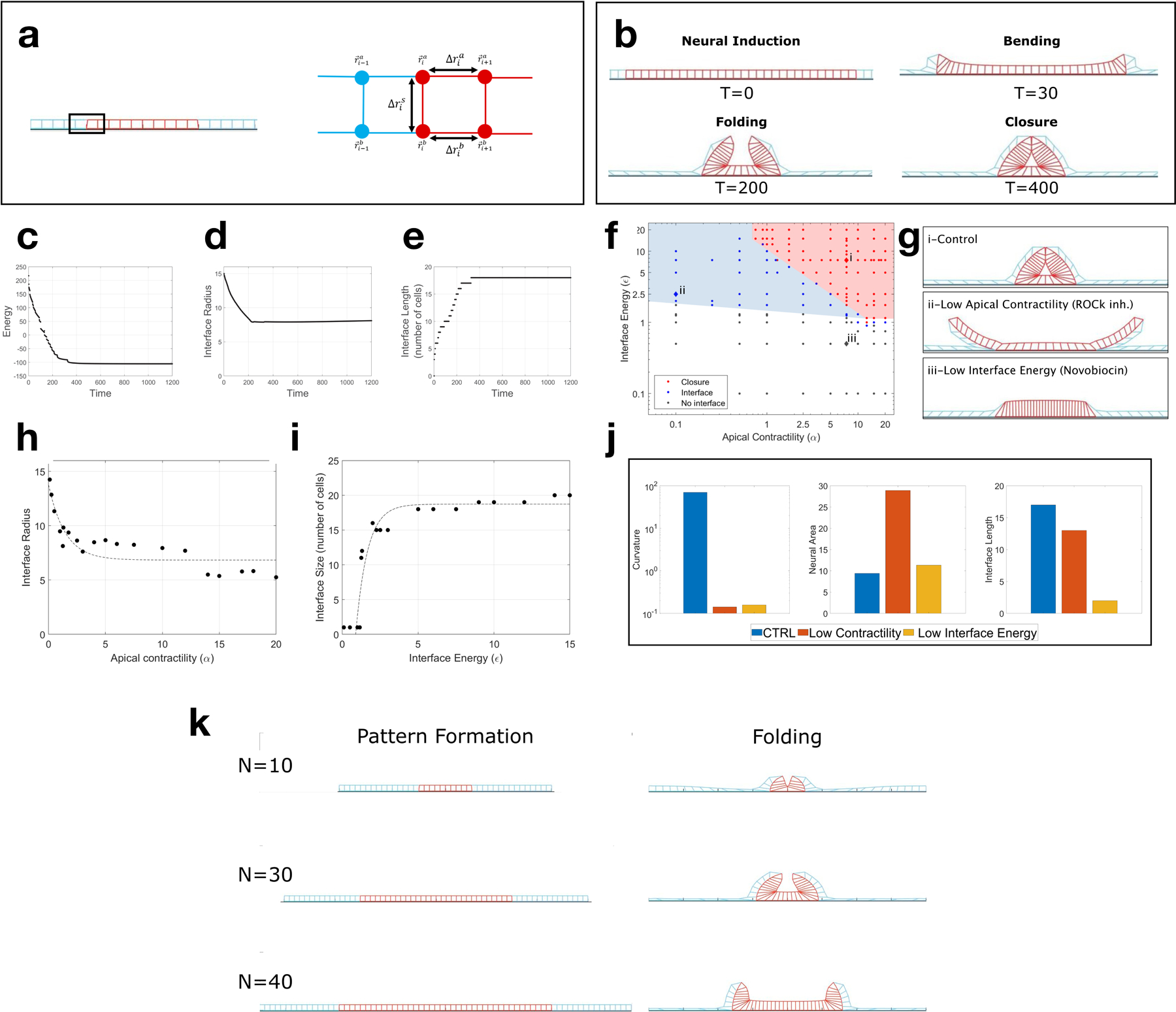
(a) Vertex model scheme. Vertices are connected by Hookean springs of length $\Delta r_i$. ${\overrightarrow{r}}_i^a$ and ${\overrightarrow{r}}_i^b$ are the apical and basal vertices (x and z) of cell i. Neural cells have additional myosin dependent positive apical line tension, and there is a negative line tension between neural and non-neural basal surfaces (see Supplementary Notes details). (b) Time sequence of simulation showing initial cell pattern (neural tissue in red, non-neural in blue), followed by neural bending, folding and hinge formation, and closure. Each time unit corresponds to 1000 steps in the simulation. Apical lines in the neural domain strongly contract due to myosin, but never reach zero values. (c) Energy of the tissue reduces over time and reaches a minimum. (d) Interface radius and (e) Number of cells on the interface as a function of time. Both reach a steady-state value. (f) Phase diagram of the dimensionless parameters interface energy ($ϵ$), neural contractility (α). Each point represents a simulation that reached a steady state. Color code represents the final configuration of the simulations: neural fold closed (red), formation of neural/non-neural interface without closure (blue), and no interface formation (black). Shaded colors were drawn by hand to highlight regime boundaries. (g) Final configuration images (steady state shapes) from the simulation in different regions i) high neural apical contractility and high interface energy leads to a closed fold; ii) Low neural apical contractility and high interface energy leads to the formation of the interface but an open fold; iii) High neural apical contractility and low interface energy leads to a flat tissue. (h) The interface radius of curvature as a function of neural apical contractility. (i) The number of cells in an interface as a function of interface energy. (j) Bar plots showing the neural apical curvature, neural apical area, and interface size for the three conditions whose final configuration are shown in g. (k) Three simulations with a 40 non-neural cells , and a varying number of neural cells N=10,30,40. Left: images of the simulation at time zero. Right: Images of the simulation at the hinge formation stage. Images were taken at this stage for consistency with experimental data (Fig. 4d, 72hrs). We observe the formation of a single hinge point for N=10, and two lateral hinges for N=30,40.