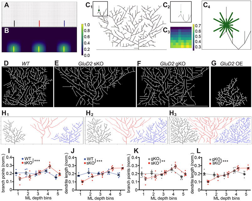
Figure 8. A Generative Model Recapitulates Key Aspects of Experimental Data.
(A) Skeleton of trees that the model begins with. Each node, denoted by a circle and representing a parallel fiber, is marked occupied when the tree extends a branch through that point on the 2D lattice. This branch (edge) is indicated by a solid line, and the color of the line indicates which tree the edge belongs to (black, red, and blue for the left, middle, and right tree, respectively). Other potential nodes for synapses are marked gray. Occupied nodes contribute to repulsion felt in that part of the grid (STAR Methods).
(B) Heat map of repulsion throughout the 2D grid shown in (A) with brighter colors indicating stronger repulsion, which discourages growth. For a given cell, the repulsion from nodes occupied by neighboring cells are stronger than repulsion from nodes occupied by itself. Color bar indicates amount of repulsion normalized to the largest value of repulsion in this heat map.
(C) Example of a decision a cell might make about whether to branch from a certain point, with eligible directions of branching indicated. (C1) A Purkinje cell with a decision point for branching denoted by the green circle. Color bar indicates amount of repulsion normalized to largest value of repulsion in this heat map. (C2) The vicinity of the green node shown in (C1). (C3) A heat map of the repulsion around the green node, which determines the probability of branching in each direction. (C4) Eligible directions for branching from the central node marked by green edges. Note that some of these directions will have 0 probability of branching if they result in crossings with current branches, but all are pictured. The endpoint for each direction is determined by the closest lattice point in that direction; because this introduces different lengths, the probabilities of branching in longer directions are adjusted accordingly.
(D) Representative example of a simulation with three wild-type Purkinje cells, showing the middle cell only.
(E) Representative example of a simulation with one GluD2 knockout Purkinje cell and two neighboring wild-type cells on either side, showing the middle cell only. This mimics the sKO condition.
(F) Representative example of a simulation with three GluD2 knockout Purkinje cells, showing the middle cell only. This mimics the gKO condition.
(G) Representative example of a simulation with one GluD2 overexpressing Purkinje cell and two neighboring wild-type cells on either side, showing the middle cell only. This mimics the OE condition.
(H1–H3) In-progress simulation at iteration 600 (H1), 800 (H2), and 1400 (H3) with one GluD2 knockout Purkinje cell (red) and two neighboring wild-type cells on either side (black and blue). Note that there is an expansion step between iteration 800 (H2) and 1400 (H3).
(I, J) Mean (± SEM) normalized dendritic branch points (I) and length (J) of bins in the molecular layer for wild-type (blue) and GluD2 sKO (red) conditions.
(K, L) Mean (± SEM) normalized dendritic branch points (I) and length (J) of bins in the molecular layer for sKO (red) and gKO (gray) conditions.
For panels I–L, data are mean ± SEM; n = 6 for all three conditions; ** p<0.01; ***p < 0.001; two-way ANOVA.

