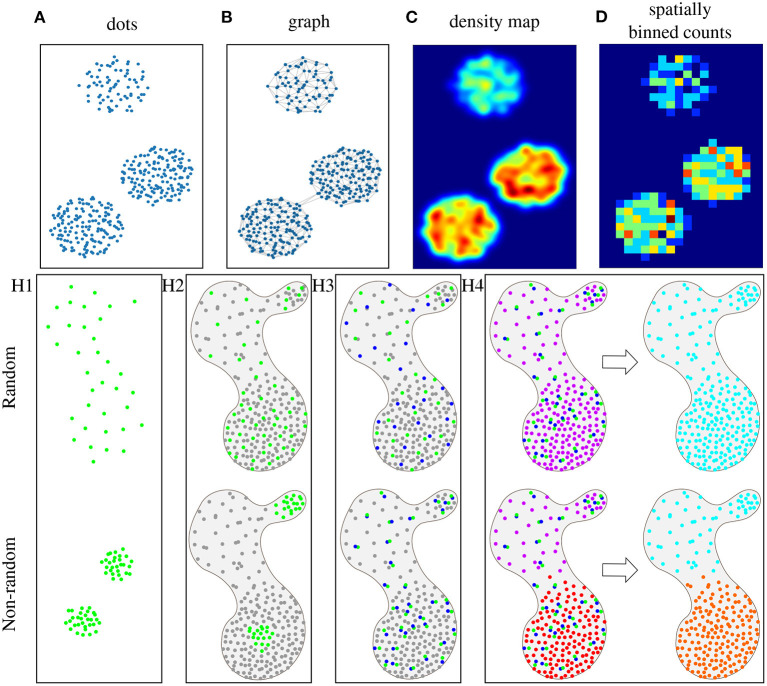
Figure 1.

Schematic representations of objects, such as cells or mRNAs, in microscopy images, where each dot represents an object, and the color reflects the object type (where gray is an unspecified type). (A) Simple representation, where each dot has a specific location in 2D tissue space. (B) The same data represented as a graph, where each dot is a node, and nodes are connected based on a maximum distance criterion. (C) Dots can also be represented by a probability density map, where warmer colors represent more dense dots, or (D) as counts in fixed spatial bins. Here, bins are squares and warmer colors represent higher object counts per bin. Spatial statistics are used to prove four different hypothesis (with the top row representing the random case): (H1) Visualization of hypothesis H1: Objects of type A (green) are non-randomly distributed. (H2) Visualization of hypothesis H2: Objects of type A (green) are non-randomly distributed as compared to the distribution of other objects (gray) in the same tissue sample. (H3) Visualization of hypothesis H3: Objects of type A (green) and B (blue) are non-randomly distributed in relation to one another within the distribution of other objects (gray) in the same tissue sample. (H4) Visualization of hypothesis H4: There are groups of object types (multiple colors in “niches”) that are non-randomly distributed within the tissue sample.