Mix Contrast for COVID-19 Mild-to-Critical Prediction

Abstract

Objective: In a few patients with mild COVID-19, there is a possibility of the infection becoming severe or critical in the future. This work aims to identify high-risk patients who have a high probability of changing from mild to critical COVID-19 (only account for 5% of cases). Methods: Using traditional convolutional neural networks for classification may not be suitable to identify this 5% of high risk patients from an entire dataset due to the highly imbalanced label distribution. To address this problem, we propose a Mix Contrast model, which matches original features with mixed features for contrastive learning. Three modules are proposed for training the model: 1) a cumulative learning strategy for synthesizing the mixed feature; 2) a commutative feature combination module for learning the commutative law of feature concatenation; 3) a united pairwise loss assigning adaptive weights for sample pairs with different class anchors based on their current optimization status. Results: We collect a multi-center computed tomography dataset including 918 confirmed COVID-19 patients from four hospitals and evaluate the proposed method on both the COVID-19 mild-to-critical prediction and COVID-19 diagnosis tasks. For mild-to-critical prediction, the experimental results show a recall of 0.80 and a specificity of 0.815. For diagnosis, the model shows comparable results with deep neural networks using a large dataset. Our method demonstrates improvements when the amount of training data is small or imbalanced. Significance: Identifying mild-to-critical COVID-19 patients is important for early prevention and personalized treatment planning.

I. Introduction

The corona virus disease 2019 (COVID-19) has caused serious public health safety problems and has become a global health emergency [1]. Five percent of the COVID-19 patients who are first diagnosed with a mild illness may become critical in the future. Moreover, this high-risk group of potentially critical patients have a very high mortality rate (approximately 49%) [2]. Thus, identifying these high-risk patients—who may change from mild to critical illness—is of great importance for early prevention and personalized treatment planning.

In current studies, clinical characteristics such as demographics, symptoms, and laboratory results have been used to predict COVID-19 patients who may change to a severe or critical state in the future [3]. For example, Liang et al. build a clinical risk model based on a large dataset of clinical characters to predict the occurrence of critical illness with an area under the curve (AUC) of 0.88 [2]. Recently, using computed tomography (CT) images for COVID-19 analysis has shown promising results. For example, CT images have demonstrated much higher sensitivity than reverse transcription polymerase chain reaction (RT-PCR) methods in diagnosing COVID-19 [4], [5]. Consequently, a study have designed prognostic models using CT images and deep learning to predict COVID-19 patients who may become severe or critical [6]. In these studies, severe and critical patients are not separated. However, critical patients have a very high mortality rate compared to severe patients. Therefore, focusing on predicting patients who may change from mild to critical is more important in clinical practice.However, it is difficult to systematically collect a large CT dataset, and the characteristics of the imbalanced small data (nearly 5% critical patients/positive samples) make the research difficult. To address this problem, we adopt contrastive learning, which has recently shown progress in few-shot learning [7] and unsupervised learning methods [8]. These methods learn representations from pairwise data instead of a single sample and include three important components: 1) Sample pairing: an image or feature (anchor) is paired with multiple images or features (supports), respectively. In this process, the anchor should be similar to the supports in the same category and dissimilar to the supports in different classes. 2) Feature distance metric: distance measurements such as the cosine distance are usually used to measure the similarity of paired samples in an embedding space. 3) Pairwise loss: unlike commonly used cross-entropy loss or mean square error loss (MSE) methods, which measure the predictive performance of a deep learning model, pairwise loss is used to measure the relative distance between two paired features. This strategy of learning the similarity between samples is suitable for small samples and imbalanced samples.

Despite the advantage of contrastive learning, directly using it in our imbalanced small data task leads to the following challenges: 1) In contrastive learning, contrastive power improvement requires many negative pairs (sample pairs from different classes) [9]. However, due to the highly imbalanced characteristics of our dataset, each sample from the majority class can only generate relatively few negative pairs. 2) Data imbalance leads to an extreme imbalance of positive pairs (sample pairs from the same class). Each sample from the minority class can only generate small numbers of positive pairs. In comparison, samples from the majority class generate large amount of positive pairs that show a large diversity, making the learning process more difficult. 3) Most contrastive networks and few-shot models usually adopt a fixed metric or calculate the dot product between two features. Some methods, such as the relation network method [7], provide a learnable metric that shows better results. However, feature combinations used for 3D image features do not satisfy the commutative law, which may limit the performance and robustness of the model. 4) Due to the highly imbalanced class distribution, many positive pairs include anchors from the majority class, whereas few positive pairs include anchors from the minority class. Commonly used loss functions tend to classify the input sample pair into one class.

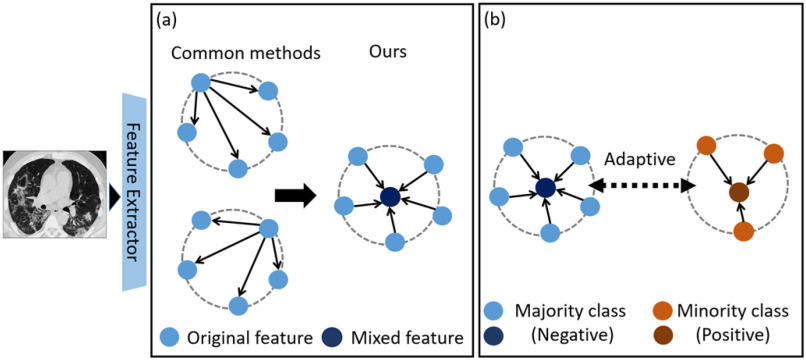
To address these problems, we propose the Mix Contrast (MixCo) method for the learning of imbalanced small data (Fig. 1). The MixCo model trains a contrastive network by matching original features with mixed features. 1) For the minority class, abundant mixed images are synthesized, which provide many negative pairs for the majority class. 2) Feature prototype (the mean of original features; used as an anchor) can represent the cluster center of the original features, and so can guide the network to learn a compact intra-class feature space. However, in the initial stages of training, the feature is not discriminative, and the mean feature is not representative. Therefore, we design a cumulative learning strategy (CLS) to gradually change the anchor from one sample of the original feature space to the mean feature. 3) Moreover, we adopt a learnable metric and propose a commutative feature combination (CFC) to learn the commutative law of feature concatenation to ensure that the network inference is not affected by the feature concatenation order. 4) Finally, we propose a united pairwise loss (UPL) to maximize the margin between classes. Based on the source of the anchors (positive or negative), we divide sample pairs into positive-anchor and negative-anchor pairs. The UPL assigns an adaptive weight for positive-anchor and negative-anchor pairs based on their current optimization status. The contributions of this work can be summarized as follows:

• 1)We propose a novel MixCo model for the classification of imbalanced small data, which pairs original features with mixed features for contrastive learning. The mixed feature guides the network to learn a compact intra-class feature space. In addition, UPL is proposed to maximize the margin between classes, assigning adaptive weights for sample pairs with different class anchors based on their current optimization status.
• 2)For efficient MixCo training, we propose a novel CLS to adjust contrastive learning, which is coupled with the MixCo model's training. In addition, a CFC is proposed to learn the commutative law of feature concatenation, which enhances the model's robustness.
• 3)We evaluate the model on the COVID-19 mild-to-critical prediction dataset to effectively predict patients who might progress to critical illness. To demonstrate the versatility of the method, we also use it for COVID-19 diagnosis and validate its performance on the diagnostic dataset. Moreover, we evaluate the performance of MixCo for different training data sizes.

Fig. 1.

Mix Contrast (MixCo) trains a contrastive network by matching original features with mixed features. a) Different from existing methods that randomly select a sample as anchor and match it with other samples, we synthesize an anchor in the embedding space, which is a mixed feature map of the original features in each mini-batch. The mixed anchor guides network efficiently learning a compact intra-class feature space. b) A united pairwise loss is proposed to maximize the margin between classes, which assigns an adaptive weight for positive-anchor pairs and negative-anchor pairs according to their current optimization status.

II. Related Work

This work draws on existing literature in contrastive learning, mixup, metric based few-shot learning, and pairwise loss. Owing to the large amount of literature, we have focused on the most relevant papers.

A. Contrastive Learning

Contrastive learning has recently shown encouraging progress in presentation learning in both self-supervised and supervised settings. These methods learn representations from pairwise data in which anchors are paired with support samples, and they are designed to minimize contrastive loss [10]. Given an anchor point, the loss forces it to be similar to the matching points (positive pairs) and dissimilar to the others (negative pairs). In the self-supervised setting, there are mainly three contrastive loss mechanisms, including end-to-end update by back-propagation [11], memory bank [12], and momentum contrastive [8]. These mechanisms differ in the maintenance method of the supports and the updating method of the encoder network [8]. In particular, the momentum contrastive method enables the building of a large and consistent dictionary on-the-fly that facilitates contrastive unsupervised learning, and the introduction of a queue decouples the dictionary size from the mini-batch size.

However, self-supervised methods need to use a large batch size and build a large memory or dictionary, which is not suitable for our task. Moreover, in the supervised setting, contrastive learning leverages label information and demonstrates more effective learning than cross-entropy. The key difference between supervised contrastive and self-supervised contrastive is the positive pairs. Specifically, the self-supervised contrastive uses only one positive pair per anchor, and the matching samples are generated as data augmentations of a given sample (crops, flips, color changes, etc.), whereas the supervised contrastive considers many positive pairs per anchor. Khosla et al. [9] combine the advantage of using labels and contrastive losses, and consistently outperform cross entropy on supervised learning tasks. Moreover, many key components facilitate contrastive learning, such as data augmentations, normalized embedding, large batch sizes, and more training steps. Our work is most related to the supervised contrastive [9]. Similarly, we only contrast samples in the current mini batch instead of building a memory or dictionary. In addition, we use many positive pairs and negative pairs per anchor instead of only one positive pair per anchor.

B. Mixup

Mixup [13] applies the interpolations of samples to regularize the neural network, which improves the generalization of the convolutional neural network (CNN) and increased its robustness to adversarial examples. Specifically, the mixed sample generated by Mixup is a convex combination of pairs of examples and their labels. The following studies further explore linear interpolations of the embedding space [13], patch mixing [14], and rebalanced Mixup strategies [15], which show significant improvement over Mixup itself. Mixup has also been widely used in other learning tasks such as semi-supervised learning [16], neural network calibration [17], and adversarial defense [18]. Mixup is commonly used to generate new samples using data augmentation. In this study, we synthesize a mean feature map of the original feature maps with the same class using Mixup. The mean feature map represents the cluster center of the original features, which is used as an anchor for contrastive learning, and proved to be better than using a random feature map as an anchor.

C. Metric-Learning-Based Few-Shot Learning

Metric learning is used to learn a high-dimensional embedding space, the similarity of sample pairs being measured in the embedding space. In the few-shot learning setting, the testing points are compared to few-shot labeled training points and recognized using classifiers or nearest-neighbor methods. Siamese networks [19], matching networks [20], and prototypical networks [21] use a linear classifier or fixed nearest-neighbor method to calculate similarity. Instead of using a fixed metric, a relation network [7] and a cross attention network [22] define a relation classifier with a CNN, providing a learnable metric. Similar to the relation network approach, This study adopts a CNN (Compare Net) to achieve an adaptive metric. Moreover, we propose a CFC to learn the commutative law of feature concatenation to ensure the inference of Compare Net is not affected by the feature concatenation order.

D. Pairwise Loss

To maximize the within-class similarity and minimize the between-class similarity, we use pairwise loss to optimize the CNN. It includes triplet loss, self-supervised contrastive loss, supervised contrastive loss, and circle loss [23]. The key distinction among these methods is the number of positive and negative pairs considered in an anchor. The triplet loss uses only one positive and one negative pair. Self-supervised contrastive losses use only one positive pair selected by co-occurrence [8] or data augmentation [24], and use enormous negative pairs. In the supervised contrastive loss, the positive pairs are chosen from the same class, and the negative pairs are chosen from other classes using hard-negative mining [25].

III. Methodology

In this paper, we attempt to leverage contrastive learning methods in situations with extremely imbalanced medical image classification and few positive samples. To achieve this goal, we propose the MixCo and several essential components: CLS, CFC, and UPL. This method includes three parts, as shown in Fig. 2.

• 1)Image preprocessing and mixed-positive sample generation: here the original CT images are preprocessed before being fed into the CNN; mixed-positive samples are generated by interpolating linearly any two positive samples.
• 2)Feature extraction and combination: positive and negative samples are fed into the encoder network to generate support features. The anchor of each class is generated on-the-fly in the embedding space, which is a mixed feature map of the same class of support features in each mini batch. During this process, a CLS is proposed to adjust the synthesis of the mixed feature. In addition, feature combinations between the anchor and support feature must satisfy commutative law.
• 3)Contrastive learning and UPL: the combined feature map is fed into the compare network to produce a similarity score, and the UPL assigns an adaptive weight for positive-anchor pairs and negative-anchor pairs based on their current optimization status. The components are described in detail in the following subsections.

Fig. 2.

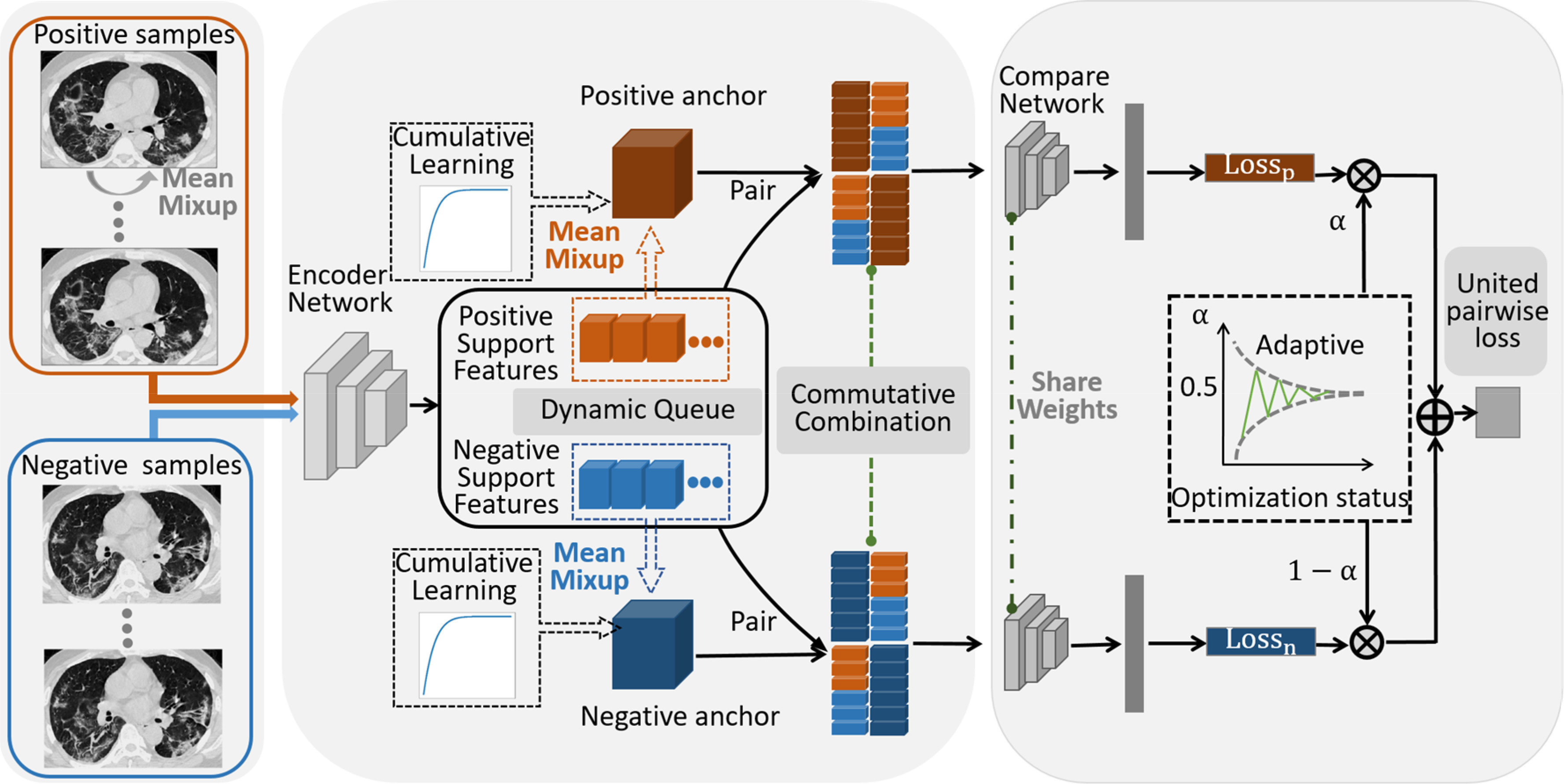
Framework of the MixCo network. It consists of three parts: 1) Image preprocessing and mixed samples generation: mixed samples are generated by interpolating linearly any two samples in the same class for minority class (positive) samples. 2) Feature extraction and combination: positive and negative samples are input to the encoder network to generate support features, and the support features are maintained as a dynamic updated queue. A positive (negative) anchor is generated on-the-fly in the embedding space, which is a mixed features of positive (negative) support features in each mini-batch. A CLS is proposed for synthesizing the mixed feature and to adjust contrastive learning. In addition, feature combinations between anchor and support features must satisfy commutative law. 3) The compare network and united pairwise loss: the combined feature map is fed into the compare network to produce a similarity score, and the UPL assigns an adaptive weight for positive-anchor pairs and negative-anchor pairs based on their current optimization status.

A. Image Preprocessing and Mixed-Positive Sample Generation

1). Image Preprocessing

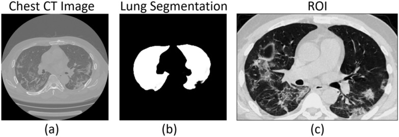
The original CT images should be preprocessed before being input into the CNN. The preprocessing standardizes the regions of interest (ROIs) of the CT images and stabilizes the prediction model. The preprocessing procedure consists of three steps, including lung segmentation, ROI acquirement, and normalization (Fig. 3).

Fig. 3.

ROI acquirement procedure. The lung ROI is cropped from the original CT images based on the lung segmentation results.

a). Lung Segmentation

A deep learning segmentation model based on DenseNet121-FPN [26] is trained on the VESSEL12 dataset [27]. It can automatically segment the lung region from the original CT image to acquire the lung mask.

b). ROI Acquirement

The cubic bounding box of the segmented lung mask is used as the ROI to crop the lung area in the original CT image. The lung ROI includes the lung areas and inflammatory tissues attached to the lung wall. The lung ROI is shown in Fig. 3(c).

c). Normalization

The three-sigma rule of thumb is used to exclude abnormal values of the CT images, which suppresses the intensities of non-lung areas inside the lung ROI. Afterwards, the lung ROI is resized to 240 × 360 × 48 and standardized using z-score normalization, making all the image intensities inside the ROI consistent, obeying a normal distribution.

2). Mean Mixup and Mixed-Positive Sample Generation

We resort to Mixup to expand the minority class (positive) samples in our data. Different from the traditional Mixup method, which interpolates linearly random images or features, we define mean Mixup interpolating linearly two images or multiple features with the same class label. To simplify the calculation, mean Mixup performs element-wise mean operation of images or features. We apply mean Mixup to the positive samples for generating mixed-positive samples. For example, we randomly select two samples (, Fig. 4(b), (c)) from the positive sample set and perform the mean Mixup procedure to generate a mixed-positive sample , as shown in Fig. 4(a). Thus, the label is unchanged.

Fig. 4.

Mixed-positive image is the linear interpolation of any two original positive images.

3). Support Features as a Queue

For MixCo's stable training, we maintain the support features as a feature queue. The queue is dynamic, and the features in the queue are progressively replaced. For every class, the current feature is queued, and the oldest feature in the queue is removed. The queue size is always a typical mini-batch size instead of building a dictionary [8] or a large memory bank[12]. Moreover, the mixed anchor is generated by the features in the queue, and slowly updated the queue making the anchor consistent during training.

B. Feature Extraction and Combination

We construct an encoder network to extract the features of samples. Subsequently, the support features are combined with an anchor to build combined features, which are input to the compare network for further analysis.

1). Encoder Network

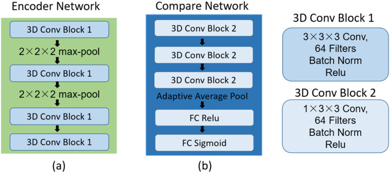
The encoder network aims to learn a projection function and map images to an embedding space. The network has a similar architecture to that of [7], as shown in Fig. 5(a). The network contains four 3D convolutional blocks, each of which is composed of a 3D convolution layer (kernel size, 3 × 3 × 3), a 3D batch-normalization layer, and a rectified linear unit (ReLU) nonlinearity layer. The max pooling layer is used to down-sample the feature maps generated from the 3D convolutional blocks. The batch-normalization layer is used to normalize the feature map output from each convolution layer—this is beneficial to the subsequent contrastive learning for analyzing the small difference between feature maps.

Fig. 5.

Network parameters of the encoder network and compare network.

2). Anchor Generation With a Cumulative Learning Strategy

By intuition, if an anchor is the cluster center of one class of features, using contrastive learning, the network may force the features to maintain a small distance from the anchor. This means that the features will be close to each other, that is, the features will have a compact intra-class feature space. Consequently, we try to build an anchor representing the cluster center for the features of each class. Similar to k-means algorithms [28] that set the cluster center at the centroid of the corresponding cluster, we synthesize a mean feature for each class of features as the cluster center. During training in each mini-batch (batch size of each class is b), the mean feature is generated on-the-fly using the mean Mixup in the embedding space:

However, in the initial stages of training, the image feature is not discriminative; hence, the mean feature is not representative. Similar to k-means, which randomly selects K samples as the initial cluster centers, we randomly select a feature of the sample as an anchor. Besides, we propose a CLS for gradually shifting the anchor from the feature of a random sample in each training batch to the mean feature. By controlling the weights for andwith an adaptive trade-off parameter , the weighted feature map and are integrated as an anchor feature map . The output anchor is formulated as:

The in the CLS is automatically generated based on the training epoch. Specifically, the number of total training epochs for cumulative learning is denoted by and the current epoch by T. is calculated by:

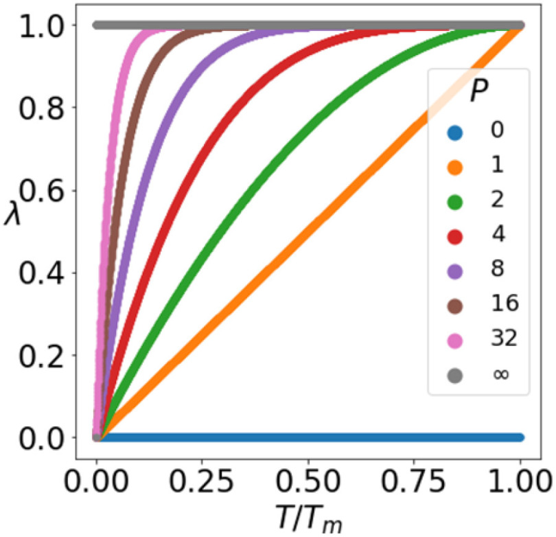
where gradually increases as the number of training epochs increases. The anchor is initialized using the feature of a random sample and then gradually shifts to the mean feature. As shown in Fig. 6, when the parameter is 0 or infinity, the strategy is named as No-mix or All-mix, respectively. Other strategies are (0 < p < ∞)exponent increments with different growth rates.

Fig. 6.

Adaptive strategy with different parameter for generating .

3). Commutative Feature Combination

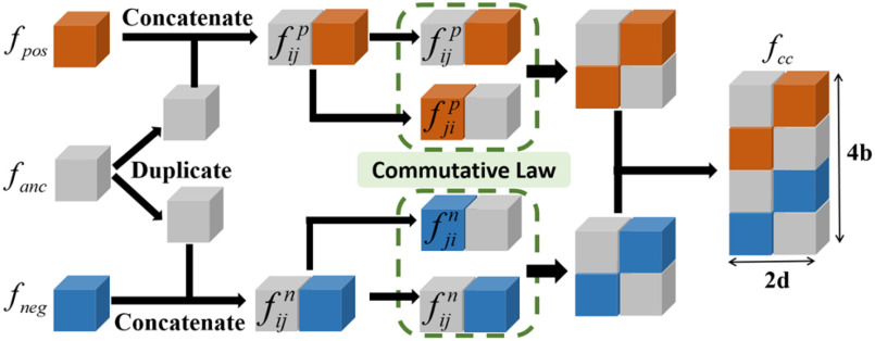
For a learnable metric, the anchor and support features are combined before being fed into the compare network. Here, we assume the feature combination to be a concatenation of feature maps in depth. In our observation, when we exchange concatenation order, the output of the compare network varies (Section V-A). To ensure that the feature combination satisfy the commutative law for a consistent prediction, we propose a CFC operator, which puts two combined features that satisfy the commutative law of concatenation order into one training batch. It contains two parts: a pairing unit and an exchange unit: (i) The pairing unit pairs the anchor with support features (including positive and negative features) and concatenates C_d(.) to the pairwise feature maps f(x_i) and f(x_j) in depth as a combined feature map:

(ii) The exchange unit first exchanges the concatenation order of to build a new feature map:

Combining the combination feature maps every class ( and; k = 1, 2,… K, K represents the class number) in batches as a commutative combination feature :

Under the toy scenario, where there is only a single anchor and a pair of positive and negative features, the function of the CFC is shown conceptually in Fig. 7. The outputs from the encoder network are feature maps of, , and , and each has a size of with c channels, d depth, l length, w width, and h height. The pairing unit first duplicates and then concatenates it with and, respectively, to form two combined feature maps (and ) of size . Subsequently, the exchange unit exchanges the concatenation order in the combined feature map to build new feature maps ( and). Finally, four feature maps (, , , and ) are put into one training batch. In this toy scenario, the final commutative combination feature is , a tensor of size .

Fig. 7.

Pairing and combining of an anchor with positive and negative feature maps to generate the commutative combination feature .

C. Compare Network and Pairwise Loss

1). Compare Network

The combined feature map is further fed into the compare network with calculating the similarity score of the pairwise samples. The anchor feature is compared with the features of the support samples by the compare network, and it yields a similarity score ranging from 0 to 1, determining whether they are from the same category or different category. As shown in Fig. 5(b), the network contains three 3D convolutional blocks, one adaptive average pooling layer, and two fully connected layers. A sigmoid function transforms the output of the last fully connected layer to a similarity score. Similar to the encoder network, each block is composed of a 3D convolution layer, a 3D batch-normalization layer, and a ReLU activation layer. The 3D convolutional kernel size of is used in the convolution layer, which is different from that in the encoder network.

2). United Pairwise Loss

The pairwise loss aims to maximize the within-class similarity and minimize the between-class similarity . Given an anchor, we assume that there are K within-class similarity scores and L between-class similarity scores, which are denoted as {} (i = 1, 2,.., K), and {} (j = 1, 2,.., L), respectively. Sun et al. [23] propose a unified loss function (9) for metric learning with class-level labels and with pair-wise labels to minimize each as well as to maximize . The unified loss tries to make the smallest greater than the largest . Based on this unified optimization target, we define a unified optimization distance to measure the optimization status for different pairwise losses, and set the margin item margin (m) to be 0.5.

When the pairwise loss is applied to imbalanced data, the optimization distance for different categories of anchor (, k = 1, 2,.., K) is different; however, they are equal in optimization. Thus, we propose a UPL that unites the optimization of sample pairs with different categories of anchor. The union loss is the weighted sum of the pairwise loss with different category anchors, which dynamically balances the optimization depending on their current optimization status. Here, we define:

In the experiments, when the positive pairs deviate too far from the optimization distance of negative pairs (), a large weighting factor has to be obtained to achieve an effective update with a large gradient. The loss is calculated based on conventional classification loss (MSE and focal loss) and pairwise loss, such as triplet, supervised contrastive loss and circle loss.

3). Inference Phase

In the inference phase, the training set is used as the support set. Given a testing case , the similarity scores between and the support samples are calculated as . Specifically, (G is the MixCo model, is the i-th sample in the sample set with label k). The category of is judged by the mean similarity score and belongs to the category with the highest mean score.

In the experiment, the predicted category is:

IV. Experiments

A. Evaluation Datasets and Empirical Settings

In this section, we present the image datasets used in the experiments.

1). Patient Database

A total of 918 patients from four hospitals participated in this study, including 559 patients from the Renmin Hospital of Wuhan University (Center 1), 113 patients from the Henan Provincial People's Hospital (Center 2), 98 patients from the Beijing Youan Hospital (Center 3), and 148 patients from the 2^nd Affiliated Hospital of the Harbin Medical University (Center 4). This multi-center retrospective study was approved by the Institutional Review Board of the four hospitals, and the requirement for informed consent was waived.

2). Mild-to-Critical Illness Prediction Dataset

In the mild-to-critical prediction task, data of 457 COVID-19 patients from Center 1 were used, including that of 50 patients who finally changed from mild to critical (Table I). In many studies, the ratio between the training (including validation samples) and testing sets is set at a ratio of 7:3 or 8:2, hence we follow this setting to split the data of the majority class. However, since the data of the minority class are small, the ratio of 7:3 or 8:2 will lead to a very small testing set in the minority class. Consequently, according to the data amount, we split the data of minority class at a ratio of 2:1 or 3:1. Due to imbalanced distribution, the data of the majority class were randomly split into training (n = 326) and testing (n = 81) sets at a ratio of 8:2. Since there are only 50 positive samples (minority class), we used two-fold cross-validation to evaluate the performance of the proposed method and used an early stop strategy during the training model. Lastly, the proportion of positive samples in the training set is 0.071, which gets close to the real ratio of 0.05. Before training, the CT images were preprocessed: (1) lung ROIs were cropped from the CT images and normalized, and (2) mixed-positive samples were generated.

TABLE I. Mild-to-critical Illness Prediction Dataset.

Mild-to-critical prediction dataset	Mild-to-critical	Other types
Training	25	326
Validation	25	81
Total	50	407

3). COVID-19 Diagnosis Dataset

To demonstrate the versatility of the MixCo model, we used it for COVID-19 diagnosis (identifying COVID-19 vs. other types of pneumonia) and evaluated its performance for different training data sizes. In this experiment, data of 918 patients from the four centers were used (Table II). All CT images were preprocessed, and the data of each center were split into training, validation, and testing sets at a ratio of 6:1:3. To compare the performance of the MixCo model for different amounts of training data, a subset of training data (at ratios of 25%, 50%, 75%, and 100%) were randomly extracted for experiments.

TABLE II. The COVID-19 Diagnosis Dataset.

Diagnosis dataset	Center 1	Center 2	Center 3	Center 4
COVID-19	457	65	68	71
Non-COVID-19	102	48	30	77
Total	559	113	98	148

4). Lung Nodules Classification Dataset

The public LIDC-IDRI dataset [29] includes 1010 patients (1018 scans) and we extract 2654 nodules using pylidc toolkit [30]. For each nodule, there are 1-7 radiologists drawing the contour and providing a malignancy rating score (1-5). We used the same criteria in previous study [31]–[33], where the nodules with average rating score above 3.5 are labeled as malignant and the nodules rated less than or equal to 3.5 are labeled as another class (unsure or benign). Due to imbalanced distribution, the data of the majority class were randomly split into training (including validation samples) and testing sets at a ratio of 7:3. Similar with the first experiment, we used a half of positive samples (minority class) as the testing dataset. Since there are 190 positive samples (minority class) in the training set, we use tree-fold cross-validation with 127 training samples and the mean results of three experiments are reported, as shown in Table III.

TABLE III. The LIDC-IDRI Dataset.

LIDC dataset	Malignant	Other types (Unsure and benign)
Training	127	1516
Validation	63	63
Testing	192	693
Total	382	2272

B. Model Training and Implementation Details

Batch normalization and data augmentation (random center crop) were used during training of the networks. For the MixCo models, we used Adam optimization and the initial learning rate was set to 0.01, which was subsequently reduced by a factor of 0.5 when the training loss was reduced to tenths of the previous value. The in the CLS was set to 1000, and the batch size was set to 8. A big batch size was proven to be effective in contrastive learning. However, owing to GPU memory limitations, we used a gradient averaging strategy, where one back-propagation was used after multiple forward propagation iterations. For testing, the last three results (the interval was 10 iterations) of each model are shown. To compare the performance of the MixCo model with a small training dataset, a 3D Resnet50 model was adopted, which was pre-trained using eight medical datasets [34]. We used the stochastic gradient descent (SGD) method with an initial learning rate of 10e^-2 and a momentum of 0.9 in the experiments with Resnet50.

We implemented the CNN using Pytorch [35] 1.4 on a machine running Ubuntu 16.04 with CUDA 10.0 and cuDNN. Training was performed on a 24 GB NVIDIA TITAN RTX.

V. Results

A. The Performance of MixCo in Predicting Mild-to-Critical Patients

The proposed MixCo model was benchmarked against the standard classification networks (ResNet50) with different learning strategies (resample, focal loss, and Mixup). Furthermore, the research most closely related to ours, including RelationNet and Supervised contrastive learning (SupCon) were compared. The basic MixCo model consisted of an encoder network and a compare network, and used the mixed anchor and Triplet loss methods. To validate the effects of the proposed components, including the CFC, CLS, and UPL, we added the components to the basic MixCo model one by one. In addition, all experiments used mixed-positive samples.

As shown in Table IV, the classification network with Focal loss shows a higher F1-score than the other two strategies, illustrating that reweighting strategy is useful to stop the model from classifying all samples to the majority class. SupCon shows an F1-score comparable to the Focal loss algorithm. We further validated the effectiveness of the proposed components, and the results showed that every module demonstrated an improvement.

TABLE IV. The Performance of MixCo.

Methods	Accuracy	Precision	Recall	F1-score	Specificity
Resample	74.2	56.8	54.0	49.5	80.5
Focal Loss	85.2	83.9	48.7	60.6	96.5
Mixup	85.2	97.4	38.7	54.6	99.6
RelationNet	77.7	57.6	31.3	38.2	92.0
SupCon	83.8	81.0	50.0	57.4	94.2
MixCo (Basic)	80.5	74.4	49.3	50.6	90.1
MixCo (CFC)	70.9	45.0	55.3	48.4	75.7
MixCo (CFC-CLS)	81.4	58.7	75.3	65.7	83.3
MixCo (CFC-CLS-UPL)	81.1	57.1	80.0	66.6	81.5

Using the CFC improved the recall from 0.493 to 0.553. Using the CLS with an appropriate parameter P showed better results with recall = 0.753 and specificity = 0.833. When adding the UPL strategy, the MixCo model showed the best performance with a recall of 0.8 and a specificity of 0.815.

F1-Score is the harmonic average of a trading off between precision and recall, which can comprehensively evaluate model performance, especially on the imbalanced data. In all experiments, our model shows the maximal F1-score, and it shows large improvement than other methods in terms of recall, but shows slight decrease in terms of specificity. In the COVID-19 mild-to-critical prediction task, we aim to identify high-risk patients who have a high probability of changing from mild to critical COVID-19 (only account for 5% of cases). It is important to early identify the high-risk patients and avoid missed care. Hence, recall (sensitivity) is more important than specificity. We use the Chi-square test [36] to evaluate the improvement of the MixCo model over ResNet50 (with Focal loss). The results indicate the improvement of our model on recall value is statistically meaningful (p = 0.007) and the decrease of our model on specificity value is not significant (p = 0.316).

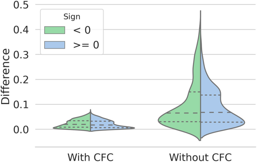
In the training dataset, due to the limited positive samples, many negative samples are paired with the same positive sample with the same combination order. Hence, the Compare Network tends to overfit. By exchanging the feature combination order, the output of the compare network varied, and the distribution of the prediction difference (with/without a CFC) is shown in Fig. 8. As expected, by using the CFC during training, the difference was small enough; that is, the compare network could apply commutative law, which enhances the model's robustness and yields a higher recall. To prove our hypotheses, we analyze the weights of the first convolution layer in Compare Network. The size of the weights is 64 × 128 × 1 × 3 × 3 and can be divided into 64 groups.

Fig. 8.

The distribution of the prediction difference.

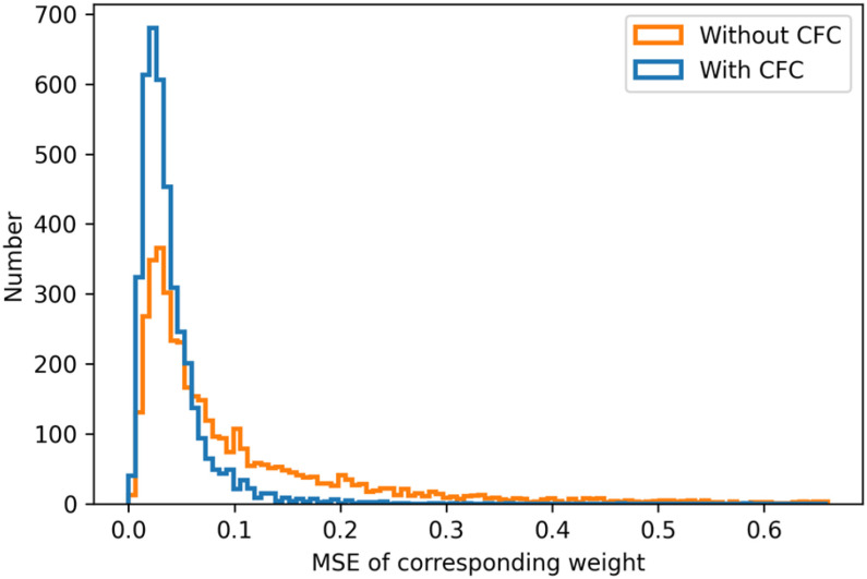
Each group consists of 128 3D convolution kernels with the size of 1 × 3 × 3. According to hypotheses, for each group, the parameters between the first 64 kernels and the last 64 kernels are commutative, hence we calculate the MSE between every two corresponding convolution kernel weights, e.g., both the first and the 64^th convolutional kernels. After calculation, we get 4096 (64 × 64) MSE values and compare the MSE values between the model with CFC (mean is 0.039) and the model without CFC (mean value is 0.107) using the T-test. The P-value in T-set is less than 0.001, which proves our hypothesis., The histogram of MSE values between the model with CFC and the model without CFC is shown in Fig. 9.

Fig. 9.

The histogram of the MSE values.

B. Different Cumulative Learning Strategies

An increment function with parameter P was proposed for the cumulative learning of the MixCo model. By adjusting the parameter P, the learning speed changes—a larger P making the anchor shift to the mean feature faster.

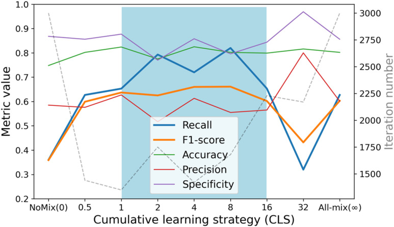
We show the change in metric values (accuracy, precision, recall, F1-score, and specificity) and the iteration number as the P value increases, in Fig. 10. Note that all experiments used the UPL approach. The results showed that using the all-mix strategy yielded significantly better performance than the no-mix strategy, which improved the recall from 0.360 to 0.627. For the exponent increment strategies, the good and stable stages (in the blue zone) are highlighted, from which we can draw three observations: 1) The MixCo model exhibits high robustness with parameter P (1 < P < 16); 2) The models using a CLS converge faster; 3) Compared to the all-mix strategy, the CLS further improves the recall of the MixCo model to 0.8.

Fig. 10.

The change of metric values (accuracy, precision, recall, F1-score and specificity) and the iteration number as the P value increases.

The NoMix strategy is based on instance discrimination (randomly select a sample as the anchor and match it with other samples), which treats two samples as a positive (negative) pair if they are from the same (different) category, regardless of their feature diversity. Hence, the paired sample shows a large diversity, making the learning process difficult. In the experiments, the number of positive sample () is 25 and the negative sample () is 326, therefore the number of paired samples is 69575 calculated according to Formula 1. In comparison, the samples are paired with the two anchors in the CLS strategy, and the number of paired samples is only 702 calculated according to Formula 2. As shown in Fig. 9, NoMix strategy needs many iteration numbers and does not converge to a stable state due to the large amount of paired samples, which is consistent with our hypothesis.

An increment function with parameter P was proposed for the cumulative learning of the MixCo model. By adjusting the parameter P, the learning speed changes—a larger P making the anchor shift to the mean feature faster, but needs more training iteration. These observations prove our motivation that in the initial stages of training, the mean feature is not representative, and leaning from the instance anchor initially is necessary for Compare Network.

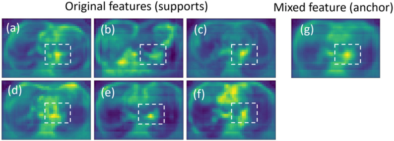
After training, the feature similarity of different samples from the same category gradually increased, as shown in the dashed box area in Figs. 11(a)–(f). The features show a similar structure and are similar to the mean feature (Fig. 11(g), anchor). The results confirmed our motivation for considering the mean feature as an anchor to guide the network to learn a compact intra-class feature space.

Fig. 11.

Examples of the mean feature and original feature. The features in the dashed box show a similar structure.

C. Advantage of the United Pairwise Loss

To prove the advantage of the proposed UPL strategy, we explored several different optimization functions. Specifically, we tested using MSE, focal loss, supervised contrastive loss (SupCon), and Triplet loss. As shown in Table V, the models

TABLE V. Effect of the UPL Strategy.

Methods	Accuracy	Precision	Recall	F1-score	Specificity
MSE	83.6	76.2	46.0	57.0	95.3
MSE (UPL)	75.6	49.3	75.3	59.4	75.7
Focal	76.6	53.9	65.3	57.3	80.0
Focal (UPL)	79.4	60.8	66.0	61.5	83.5
SupCon	78.6	58.0	65.3	58.9	82.7
SupCon (UPL)	80.2	59.1	66.0	61.5	84.6
Triplet	81.4	58.7	75.3	65.7	83.3
Triplet (UPL)	81.1	57.1	80.0	66.6	81.5

with a UPL strategy yielded better recall and F1-score results than those with the original strategy. These observations prove that the UPL strategy is effective, balancing the optimization of imbalanced data to improve the performance for minority classes. Among these strategies, the best was Triplet loss with the UPL.

D. Inference Using a Subset of Support Samples

In the inference phase, the training data are used as the support set. When the support size is large, the performance can probably improve. However, it can lead to more computational overhead and can be time-consuming. Therefore, we explored possible critical values as a trade-off. We used stratified random sampling to acquire a subset of the support data for inference. Table VI shows the prediction results of one MixCo model using different numbers of support samples. We randomly performed 10 samplings for each subset size, and the following metrics were calculated: Recall, F1 score, and Specificity.

TABLE VI. Inference Using a Subset of Support Samples.

Number	Recall	F1 Score	Specificity	Inference time (s)
5	0.704 ± 0.269	0.565 ± 0.168	0.769 ± 0.131	0.0865
10	0.780 ± 0.041	0.650 ± 0.021	0.809 ± 0.027	0.0897
15	0.788 ± 0.036	0.655 ± 0.014	0.809 ± 0.028	0.0959
20	0.792 ± 0.024	0.657 ± 0.014	0.809 ± 0.010	0.0971
25	0.800 ± 0.025	0.657 ± 0.012	0.804 ± 0.022	0.0976

The results show that a larger number of support samples yield better performance and smaller prediction variance. However, from Table VI, we can see that when the number of support samples exceeds 20, the results do not show much improvement but bring more memory usage and inference time. We use Chi-square test [36] to evaluate the results with 20 support samples and 25 support samples, and the p value is 0.854 for recall value. Therefore, we can select a small number of typical examples (n = 20) as the support set.

E. The Versatility of MixCo in COVID-19 Diagnosis

To demonstrate the MixCo model's versatility, we performed experiments on the diagnosis dataset and evaluated the performance of it with respect to different training data sizes. Table VII shows the performance of both the MixCo model and the pre-trained 3D Resnet50 model [34] for the four centers. For each center, four experiments with part of the training data (at ratios of 25%, 50%, 75%, and 100%) were used. For a fair comparison, the MixCo and 3D Resnet50 models used the same settings. Due to data imbalance in Center 1, focal loss was used for training the Resnet50 model. The following metrics were calculated: AUC, Rcall and Specificity.

TABLE VII. Comparison Between The MixCo and Resnet50 Models Regrading Different Amounts of Training Data.

Model		Ratio of data used to train model
		25%	50%	75%	100%
		AUC (Recall, Specificity)
1	MixCo	0.83 (0.88,0.53)	0.86 (0.91,0.50)	0.86 (0.86,0.63)	0.89 (0.83,0.84)
	Resnet50	0.69 (0.65, 0.73)	0.72 (0.74,0.63)	0.76 (0.93,0.53)	0.81 (0.85,0.67)
2	MixCo	0.80 (0.74, 0.71)	0.80 (0.63,0.86)	0.88 (0.79,0.79)	0.94 (0.84,0.71)
	Resnet50	0.74 (0.89,0.57)	0.78 (0.95,0.64)	0.88 (0.84,0.86)	0.90 (0.84,0.86)
3	MixCo	0.95 (0.90,0.87)	1.00 (1.00, 1.00)	0.92 (0.75, 1.00)	0.94 (0.95,0.87)
	Resnet50	0.94 (0.80,1.00)	0.95 (0.95,0.87)	0.94 (0.90,0.93)	0.97 (1.00,0.87)
4	MixCo	0.83 (0.67,0.87)	0.95 (0.81,1.00)	0.96 (0.86,1.00)	0.99 (0.95,0.91)
	Resnet50	0.74 (0.81,0.65)	0.90 (0.86,0.91)	0.89 (0.81,0.96)	0.96 (0.90,0.91)

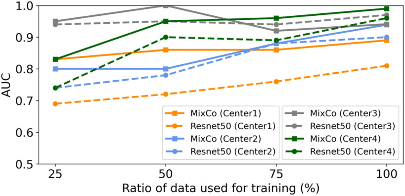
Overall, the results in the four centers were consistent, and the performances of both models improved as the amount of training data increased. When the two models were trained with 100% of the training data, they consistently had high AUCs. However, the MixCo model outperformed the Resnet50 model steadily on imbalanced data (Center 1). In addition, when the amount of training data decreased, the MixCo model showed better performance than the Resnet50 model. To provide a more intuitive comparison, Fig. 12 shows the AUC comparison between the MixCo and Resnet50 models regrading different amounts of training data. The Resnet50 model relies on large amounts of data for pre-training and transferring the model. By contrast, the MixCo model can be trained from scratch on small amounts of data. This is important for COVID-19 analysis when large labeled data are difficult to collect.

Fig. 12.

AUC comparison between the MixCo and Resnet50 models regrading different amounts of training data.

F. The Versatility of MixCo in Lung Nodules Classification

We evaluate the predictive performance between ResNet models with focal loss and our method, as shown in Table VIII. MixCo shows a higher F1-score (0.574 vs 0.508) and Recall value (0.577 vs 0.375).

TABLE VIII. The Performance of MixCo on LIDC Data.

Methods	Accuracy	Precision	Recall	F1-score	Specificity
ResNet 10	84.1	83.6	33.0	46.8	98.1
ResNet 18	84.5	79.3	37.5	50.8	97.3
ResNet 34	83.7	78.6	33.5	46.9	97.4
ResNet 50	83.9	79.6	33.3	47.0	97.7
MixCo (CFC-CLS-UPL)	81.8	57.1	57.7	57.4	88.3

G. Analysis of the Optimization Process Using the United Pairwise Loss

The UPL unites the optimization of positive-anchor pairs and negative-anchor pairs. The union dynamically balances the optimization depending on the current optimization status. For example, when the optimization of positive-anchor pairs deviates too far from that of negative-anchor pairs, the UPS assigns a larger weight to positive-anchor pairs. For simplicity, is defined as the mean of {} in each training epoch, and is defined as the mean of {}. 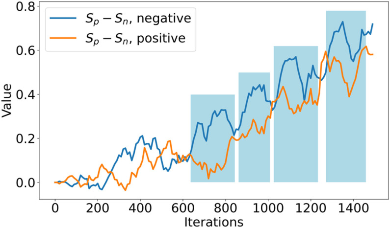To intuitively understand the optimization process, the changes in in both the positive-anchor and negative-anchor pairs during the training process, are shown in Fig. 13. At initialization, all and scores were small, and hence the values were similarly small.

Fig. 13.

The change of values of both positive-anchor pairs and negative-anchor pairs during training. We highlight the final training process (in the blue zone), and the optimization process of both change periodically.

Subsequently, the optimization of negative-anchor pairs easily dominated the training, leading to a rapid increase in the values. At this time, the UPL restrained the optimization of negative-anchor pairs and enhanced the optimization of positive-anchor pairs until in both the negative-anchor pair and the positive-anchor pair reached the same value. Consequently, the optimization process periodically changed until it converged to a stable status (as shown by the blue zone in Fig. 13).

VI. Discussion

In this work, we consider employing contrastive learning on imbalanced small data and discussed how to incorporate this idea into the early identification of high-risk patients with COVID-19 who may develop critical illness. By matching the mixed feature with original features for contrastive learning, the networks attain rapid convergence, and the mixed feature can guide network learning of a compact intra-class feature space. In the training phase, maintaining the support samples as a progressively updated queue is the key to the MixCo model's steady training. Moreover, the model design of MixCo conforms to the evidence-based medicine method. In the inference phase, each tested case is paired with the support samples to calculate the similarity scores. The category of the tested case is judged by the mean similarity score of each class and belongs to the category with the highest mean score. Hence, the cases that have been confirmed give instance-based evidence to the diagnosis, which presents good interpretability. Lastly, the MixCo model has far fewer parameters than the deep learning model, which is convenient for its use in applications.

In principle, the SupCon is the basic component of our model. Although we do not use a balanced strategy for SupCon, it shows an F1-score comparable to the best classification strategy (reweighting), as show in Table IV, which proves our hypothesis that when using the few positive samples (minority class) with large amount of negative samples (majority class) to construct sample pairs, and combined with contrastive learning can improve the model's performance of identifying positive samples. However, when we directly combine the advantages of the learnable metric in RelationNet and the contrastive learning in SupCon, the MixCo (Basic) and MixCo (CFC) show worse performances. This may be caused due to the following reason: samples from the majority class generate many positive pairs (sample pairs from the same classes) that show a large diversity, making the learning process more difficult. Hence, we design feature prototypes for each class as the anchors in contrastive learning, which guide the network to learn a compact intra-class feature space. This mechanism brings a significant improvement according to the results. Furthermore, the positive features learned by our model also focused on part of the cardiovascular system (Fig. 11), which is consistent with previous clinical findings that the cardiovascular abnormality may be a sign of fatal outcome of COVID-19. According to previous studies, COVID-19-related pneumonia can cause acute myocardial injury and chronic damage to the cardiovascular system [37], and myocardial injury is significantly associated with fatal outcome of COVID-19 [38]. Hence, MixCo model is consistent with the clinical practice [37], [38]. Besides, the proposed MixCo model aims to learn with imbalanced small data on medical image, which has two key features: (i) there are only very small amount of positive (disease) samples, and (ii) the large amount of negative samples show large diversity. Consequently, our proposed method has the potentiality to be applied in many image-based disease predictions with imbalanced class distribution, such as Alzheimer's disease diagnosis [39].

Despite the good performance of the MixCo model, this work has several limitations. First, compared with the conventional CNN model, this method needs to construct a dynamic queue and dynamic anchors of each class during training and needs extra reference data for model inference. Although our model has the merits of fewer parameters, building and saving extra intermediate data (a queue and the anchors) needs more computational resources than the conventional CNN model. Second, the fine-scale analysis for the lung region may yield better results; hence, contrastive analysis of each lung lobe and bronchopulmonary segment worth further study. Lastly, some clinical and biochemical markers are related to COVID-19 prognosis; however, we only used image information. Including more clinical and biochemical information in the system may further improve results.

VII. Conclusion

In conclusion, we propose a novel MixCo model that can be employed for imbalanced small data. We apply the MixCo model for COVID-19 mild-to-critical prediction, and it can identify high-risk COVID-19 patients who have a high probability of changing from mild to critical illness, with a high recall and specificity, which is important for early prevention and personalized treatment planning. Besides, compared with deep neural networks, the proposed MixCo model demonstrates improvements for some image-based disease predictions with imbalanced class distribution, such as COVID-19 diagnosis and lung nodule classification.

Funding Statement

This work was supported in part by the Ministry of Science and Technology of China under Grant 2017YFA0205200, in part by the National Natural Science Foundation of China under Grants 82001913 and 82001914, and in part by China Postdoctoral Science Foundation under Grants 2019TQ0019 and 2020M670101.

References

- [1].Wang C. et al. , “A novel coronavirus outbreak of global health concern,” Lancet, vol. 395, pp. 470–473, Feb. 2020. [DOI] [PMC free article] [PubMed] [Google Scholar]
- [2].Liang W. et al. , “Development and validation of a clinical risk score to predict the occurrence of critical illness in hospitalized patients with COVID-19,” JAMA Intern. Med., vol. 180, no. 8, pp. 1–9, Aug. 2020. [DOI] [PMC free article] [PubMed] [Google Scholar]
- [3].Colombi D. et al. , “Well-aerated lung on admitting chest CT to predict adverse outcome in COVID-19 pneumonia,” Radiology, vol. 296, no. 2, Aug. 2020, Art. no. 201433. [DOI] [PMC free article] [PubMed] [Google Scholar]
- [4].Wang S. et al. , “A fully automatic deep learning system for COVID-19 diagnostic and prognostic analysis,” Eur. Respir. J., vol. 65, no. 2, Aug. 2020, Art. no. 2000775. [DOI] [PMC free article] [PubMed] [Google Scholar]
- [5].Li L. et al. , “Artificial intelligence distinguishes COVID-19 from community acquired pneumonia on chest cT,” Radiology, vol. 296, Mar. 2020, Art. no. 200905. [Google Scholar]
- [6].Zhang K. et al. , “Clinically applicable AI system for accurate diagnosis, quantitative measurements, and prognosis of COVID-19 pneumonia using computed tomography,” Cell, vol. 181, no. 6, pp. 1423–1433, Jun. 2020. [DOI] [PMC free article] [PubMed] [Google Scholar]
- [7].Sung F. et al. , “Learning to compare: Relation network for few-shot learning,” in Proc. IEEE Conf. Comput. Vis. Pattern Recognit., 2018, pp. 1199–1208. [Google Scholar]
- [8].He K. et al. , “Momentum contrast for unsupervised visual representation learning,” in Proc. IEEE/CVF Conf. Comput. Vis. Pattern Recognit., 2020, pp. 9729–9738. [Google Scholar]
- [9].Khosla P. et al. , “Supervised contrastive learning,” in Proc. Adv. Neural Inf. Process. Syst., 2020, p. 33.
- [10].Hadsell R., Chopra S., and LeCun Y., “Dimensionality reduction by learning an invariant mapping,” in Proc. IEEE Comput. Soc. Conf. Comput. Vis. Pattern Recognit., 2006, pp. 1735–1742. [Google Scholar]
- [11].Bachman P., Hjelm R. D., and Buchwalter W., “Learning representations by maximizing mutual information across views,” in Proc. Adv. Neural Inf. Process. Syst., 2019, pp. 15535–15545. [Google Scholar]
- [12].Wu Z. et al. , “Unsupervised feature learning via non-parametric instance discrimination,” in Proc. IEEE Conf. Comput. Vis. Pattern Recognit., 2018, pp. 3733–3742. [Google Scholar]
- [13].Zhang H. et al. , “mixup: Beyond empirical risk minimization,” 2017, arXiv:1710.09412. [Google Scholar]
- [14].Yun S. et al. , “Cutmix: Regularization strategy to train strong classifiers with localizable features,” in Proc. IEEE Int. Conf. Comput. Vis., 2019, pp. 6023–6032. [Google Scholar]
- [15].Chou H.-P. et al. , “Remix: Rebalanced mixup,” in Eur. Conf. Comput. Vis., 2020, pp. 95–110. [Google Scholar]
- [16].Berthelot D. et al. , “Mixmatch: A holistic approach to semi-supervised learning,” in Proc. Adv. Neural Inf. Process. Syst., 2019, pp. 5049–5059. [Google Scholar]
- [17].Thulasidasan S. et al. , “On mixup training: Improved calibration and predictive uncertainty for deep neural networks,” in Proc. Adv. Neural Inf. Process. Syst., 2019, pp. 13888–13899. [Google Scholar]
- [18].Pang T., Xu K., and Zhu J., “Mixup inference: Better exploiting mixup to defend adversarial attacks,” in Int. Conf. Learn. Representations, 2019. [Google Scholar]
- [19].Koch G., Zemel R., and Salakhutdinov R., “Siamese neural networks for one-shot image recognition,” in Proc. ICML Deep Learn. Workshop, 2015. [Google Scholar]
- [20].Vinyals O. et al. , “Matching networks for one shot learning,” in Proc. Adv. Neural Inf. Process. Syst., 2016, pp. 3630–3638. [Google Scholar]
- [21].v. d. Oord A., Li Y., and Vinyals O., “Representation learning with contrastive predictive coding,” 2018, arXiv:1807.03748. [Google Scholar]
- [22].Hou R. et al. , “Cross attention network for few-shot classification,” in Proc. Adv. Neural Inf. Process. Syst., 2019, pp. 4003–4014. [Google Scholar]
- [23].Sun Y. et al. , “Circle loss: A unified perspective of pair similarity optimization,” in Proc. IEEE/CVF Conf. Comput. Vis. Pattern Recognit., 2020, pp. 6398–6407. [Google Scholar]
- [24].Chen T. et al. , “A simple framework for contrastive learning of visual representations,” in Int. Conf. Mach. Learn., 2020, pp. 1597–1607. [Google Scholar]
- [25].Schroff F., Kalenichenko D., and Philbin J., “Facenet: A unified embedding for face recognition and clustering,” in Proc. IEEE Conf. Comput. Vis. Pattern Recognit., 2015, pp. 815–823. [Google Scholar]
- [26].Huang G. et al. , “Densely connected convolutional networks,” in Proc. IEEE Conf. Comput. Vis. Pattern Recognit., 2017, pp. 4700–4708. [Google Scholar]
- [27].Rudyanto R. D. et al. , “Comparing algorithms for automated vessel segmentation in computed tomography scans of the lung: The VESSEL12 study,” Med. Image Anal., vol. 18, pp. 1217–1232, Oct. 2014. [DOI] [PMC free article] [PubMed] [Google Scholar]
- [28].Kanungo T. et al. , “An efficient K-means clustering algorithm: Analysis and implementation,” IEEE Trans. Pattern Anal. Mach. Intell., vol. 24, no. 7, pp. 881–892, Jul. 2002. [Google Scholar]
- [29].Armato S. G. III, et al. ,“ The lung image database consortium (LIDC) and image database resource initiative (IDRI): A completed reference database of lung nodules on CT scans,” Med. Phys., vol. 38, no. 2, pp. 915–931, Feb. 2011. [DOI] [PMC free article] [PubMed] [Google Scholar]
- [30].Hancock M. C. and Magnan J. F., “Lung nodule malignancy classification using only radiologist-quantified image features as inputs to statistical learning algorithms: Probing the lung image database consortium dataset with two statistical learning methods,” J. Med. Imag., vol. 3, Oct. 2016, Art. no. 044504. [DOI] [PMC free article] [PubMed] [Google Scholar]
- [31].Hussein S. et al. , “Risk stratification of lung nodules using 3D CNN-based multi-task learning,” in Proc. Int. Conf. Inf. Process. Med. Imag., 2017, pp. 249–260. [Google Scholar]
- [32].Wu B. et al. , “Joint learning for pulmonary nodule segmentation, attributes and malignancy prediction,” in Proc. IEEE 15th Int. Symp. Biomed. Imag., 2018, pp. 1109–1113. [Google Scholar]
- [33].Wu B. et al. , “Learning with unsure data for medical image diagnosis,” in Proc IEEE/CVF Int. Conf. Comput. Vis., 2019, pp. 10590–10599. [Google Scholar]
- [34].Chen S., Ma K., and Zheng Y., “Med3d: Transfer learning for 3D medical image analysis,” 2019, arXiv:1904.00625. [Google Scholar]
- [35].Paszke A. et al. , “Pytorch: An imperative style, high-performance deep learning library,” in Proc. Adv. Neural Inf. Process. Syst., 2019, pp. 8026–8037. [Google Scholar]
- [36].Agresti A., Categorical Data Analysis. New York, NY, USA: Wiley, 1990, pp. 350–354. [Google Scholar]
- [37].Zheng Y. Y. et al. , “COVID-19 and the cardiovascular system,” Nat. Rev. Cardiol., vol. 17, pp. 259–260, May 2020. [DOI] [PMC free article] [PubMed] [Google Scholar]
- [38].Guo T. et al. , “Cardiovascular implications of fatal outcomes of patients with coronavirus disease 2019 (COVID-19),” JAMA Cardiol., vol. 5, pp. 811–818, Jul. 2020. [DOI] [PMC free article] [PubMed] [Google Scholar]
- [39].Huang C. et al. , “Split LBI: An iterative regularization path with structural sparsity” in Proc. 30th Int. Conf. Neural Inf. Process. Syst., 2016, pp. 3377–3385. [Google Scholar]