. 2022 Feb 18;11:e63405. doi: 10.7554/eLife.63405

Figure 5. Bayesian model framework and correlations between the time constant and model-implied residual errors.

(A)Left: Illustration of the Bayesian estimator model. We fit two parameters: the ratio λ of standard deviations of prior and likelihood (λ=σprior/σlikelihood) and the mean of the prior (μprior) of the normally distributed variable φ=logτ (black dotted box). Likelihood function is centered on the log-transformation of the actual τ, φ*=logτ* (black dashed line). The time constant estimate τ^ corresponded to the median of the posterior distribution over τ, which corresponds to the median φ^ over φ, τ^=exp(φ^) (red dotted box;red dashed line; see Materials and methods). Middle: Control dynamics implied by the actual time constant τ (top; gray shade) and the estimated time constant τ^ (bottom; red shade). u, v, and o denote joystick input, movement velocity, and sensory observations, respectively, and subscripts denote time indices. v^ denotes the inferred velocity implied by the model. Misestimation of the time constant leads to erroneous velocity estimates about self-motion v^ which result in biased position beliefs. Right: Illustration of the actual (black) and believed (red) trajectories produced by integrating (box) the actual velocity v and the estimated velocity v^ , respectively. White and yellow dots denote the starting and target position, respectively. Inset: Illustration of correlated (black dots) and uncorrelated (red dots) residual errors with the time constant for actual and model-implied responses (simulated data). For simplicity, we depict residual errors as one-dimensional and assume unbiased responses (response gain of 1). Blown-up dots with yellow halo correspond to the actual and model-implied trajectories of the right panel. Solid black horizontal line corresponds to zero residual error (i.e. stop on target location). (B) Comparison of correlations between real and subjective residual errors with τ (Figure 5—source data 1). On the right, participant averages of these correlations are shown. Colored bars: ‘Subjective’ correlations, open bars: Actual correlations. Error bars denote ±1 SEM across participants. Asterisks denote the level of statistical significance of differences between real and subjective correlations (*: p<0.05, **: p<0.01, ***: p<0.001).

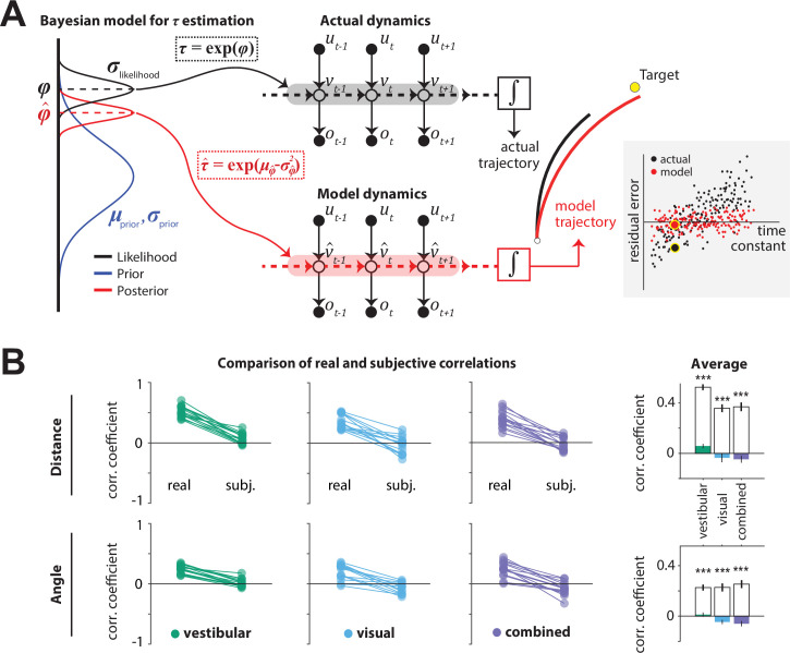
Figure 5—source data 1. correlations between time constant and model-implied residual errors.

Figure 5.

Figure 5—figure supplement 1. Testing model assumptions.

Figure 5—figure supplement 1.

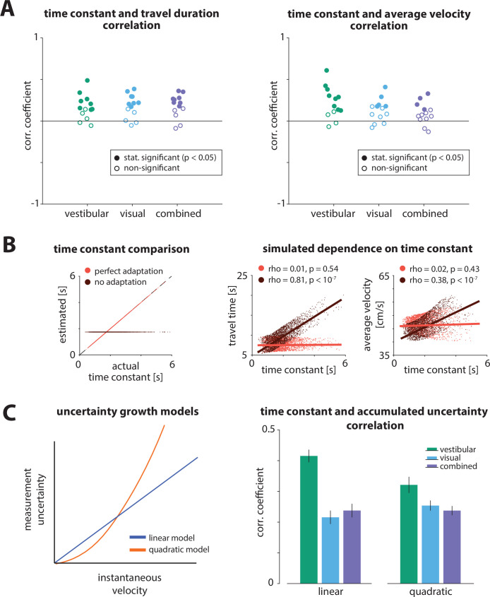
(A) Correlation coefficients between the time constant and travel duration (left) or average travel velocity (right) across trials for all participants.
Colors of circles indicate the sensory condition (green: vestibular, cyan: visual, purple: combined). Open and filled circles denote statistical significance according to the legend. (B) Dependence of travel duration (top right) and average velocity (bottom right) on the time constant for perfect or no estimation/adaptation to the dynamics (left), for a simulated bang-bang controller. Correlation coefficients and statistical significance are indicated in the legends of the corresponding panels. Solid lines represent linear regression fits. (C) Left: Uncertainty (variance) of instantaneous self-motion velocity estimation. Illustration of a linear (blue) and a quadratic (orange) model of velocity estimation uncertainty as a function of the instantaneous velocity magnitude. We wanted to test whether the effect of the time constant on performance could be attributed to differences in the accumulated uncertainty of the different velocity profiles. Right: Correlation between time constant and accumulated uncertainty for the linear and quadratic models. We found that the accumulated uncertainty is positively correlated with the time constant for both models (adding an intercept term to the models did not qualitatively change the results). This means that higher time constants yield larger uncertainty and, therefore, participants should undershoot more. However, this is the opposite of the observed effect of the time constant on the responses. Error bars denote ±1 SEM.
Figure 5—figure supplement 2. Changes in travel distance for a given control input under different control dynamics.

Figure 5—figure supplement 2.

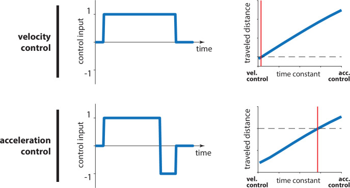
Whether in the domain of velocity (top) or acceleration control (bottom), a control input that is appropriate to reach a certain target distance (horizontal black dashed line) under only a certain time constant (red vertical line) will produce erroneous displacements under any other time constant (blue line). For smaller time constants, the intended distance will be undershot, whereas larger time constants will lead to overshooting. In other words, assuming that the red vertical line denotes the believed dynamics of a controller, a larger actual time constant (underestimation) will lead to overshooting (relative to the intended displacement; horizontal black dashed line). Inversely, overestimation of the time constant would lead to undershooting. Note that, for acceleration control, we chose a bang-bang controller such that we can demonstrate that this holds true whether there is braking at the end of the trial or not.