Figure 7. Comparison of the correlations between the actual τ and the subjective residual errors implied by three different τ-estimation models (Bayesian estimation with a static prior ([S], Bayesian estimation with a dynamic prior [D], fixed estimate [F]).

We tested the hypotheses that either the prior distribution should not be static or that the participants ignored changes in the control dynamics and navigated according to a fixed time constant across all trials (fixed τ estimate model; see Materials and methods). For this, we compared the correlations between the subjective residual error and the actual trial τ that each model produces. The dynamic prior model performs similarly to the static prior model in all conditions, indicating that a static prior is adequate in explaining our data (p-values of paired t-test between correlation coefficients of the two models: distance – vestibular: p = 0.96, visual: p = 0.19, combined: p = 0.91; angle – vestibular: p = 0.87, visual: p = 0.09, combined: p = 0.59). For visual and combined conditions, the fixed τ model not only fails to minimize the correlations but, in fact, strongly reverses it, for both distance (left) and angle (right). Since these correlations arise from the believed trajectories that the fixed τ model produces, this suggests that participants knowingly stop before their believed target location for higher time constants. Model performance was only comparable in the vestibular condition, where the average correlation of the fixed τ model (F) was contained within the 95% confidence intervals (CI) of the static prior Bayesian model (S), for both distance and angle (distance – F: mean Pearson’s correlation coefficient ρ = 0.03, S: 95% CI of Pearson’s correlation coefficient ρ = [–0.10 0.25]; angle – F: mean Pearson’s correlation coefficient ρ = –0.01, S: 95% CI of Pearson’s correlation coefficient ρ = [–0.12 0.15]). Error bars denote ±1 SEM.

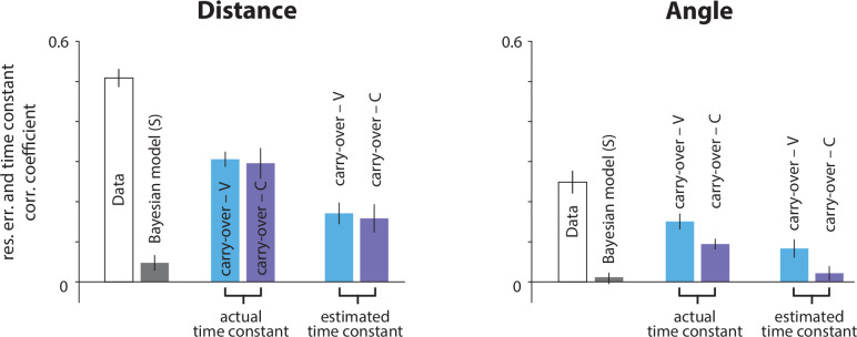
Figure 7—figure supplement 1. Correlation coefficients in the vestibular condition between the actual time constant and the subjective radial (left) and angular (right) residual errors, if participants carried over their τ estimate from the previous trial.

With sensory conditions interleaved and a common random walk of τ (see Materials and methods, Figure 1—figure supplement 3C), we searched for a trial-type history effect in the vestibular condition, due to participants’ poor τ estimation performance. Specifically, we asked whether participants in the vestibular condition would leverage from the correlation structure between recent time constants by carrying over their estimates from the previous visual or combined trials. We first compared the correlations from the actual data (open bars; same as Figures 3C and 5B) with those obtained when using the actual (middle bar couple) or estimated (right bar couple; estimates from the static prior Bayesian model) time constant from the previous visual (cyan bars) or combined (purple bars) trial to generate believed trajectories. Although correlations were significantly smaller for the carry-over models relative to the actual data (p<0.01) they nevertheless remained significant (p<10⁻⁵), thus, failing to explain away the effect (compare with gray bars: correlations implied by estimation in the current vestibular trial with the static prior Bayesian model). The carry-over strategy does not seem likely since it fails to explain away a large part of the correlation between the radial component of the subjective residual errors and the time constant (compare rightmost cyan/purple bars with gray bars; p-values of paired t-test between radial correlation coefficients – current vestibular vs. previous visual trial estimation: p=0.006, current vestibular vs. previous combined trial estimation: p=0.02; p-values of paired t-test between angular correlation coefficients – current vestibular vs. previous visual trial estimation: p=0.008, current vestibular vs. previous combined trial estimation: p = 0.71). Error bars denote ±1 SEM across participants.

Figure 7—figure supplement 2. Comparing bayesian and feedback control models.

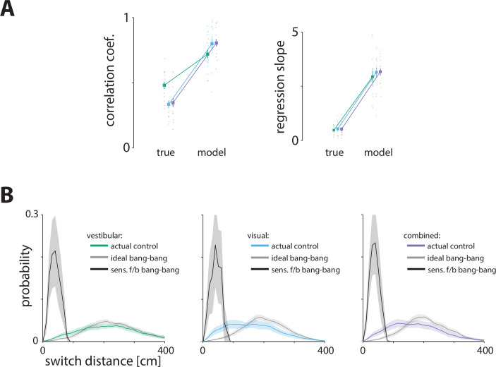
(A) We tested a sensory feedback control model, in which the controller uses bang-bang control and switches from forward to backward input at a constant and predetermined distance from the target position (corrected for the bias).

We fit the mean and standard deviation of the switch distance for each participant in each condition separately, by minimizing the distance of the actual from the model-predicted stopping locations (see Materials and methods). The correlations (left) and the regression slopes (right) between the model-predicted residual errors and the time constant were significantly higher than those found in our data (p-values of difference in correlations between true data and model obtained by paired t-test – vestibular: p = 10^–5, visual: p = 10^–6, combined: p = 10^–7; p-values of difference regression slopes between true data and model obtained by paired t-test – vestibular: p = 10^–7, visual: p = 10^–8, combined: p = 10^–9). Error bars represent ±1SEM across participants. (B) Probability distribution of bang-bang switch distance from target position (corrected for the bias). According to the sensory feedback control model, the probability distribution of switch distance should be very narrow since participants switch at a constant perceived distance from the target. If participants implemented this type of control (black lines), we would expect to see such a narrow distribution in the actual data. In all conditions, however, the switch distance distribution of the true data (colored lines) is wider and resembles what we expect to see if participants implemented optimal (ideal) bang-bang control (gray lines). Shaded regions represent ±1 SEM across participants.