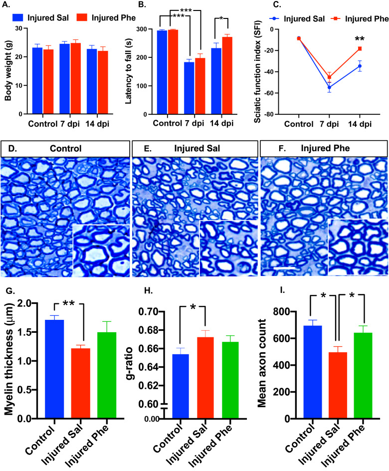
Figure 2.

Assessment of post-injury functional recovery and sciatic nerve axon morphology. (A) Mice body weights in grams (n = 8–12 per treatment group per time point). (B) Rotarod test was performed to access the motor coordination and balance of the mice before, 7 and 14-day post-injury (dpi) in mice treated with saline and phentolamine. The latency until the mice fell off the rotating rod was monitored for 300 s (n = 8–12 per group at each time point). Two-way ANOVA with Benjamini and Hochberg false discovery rate correction for multiple comparisons was performed to determine the significance. (C) Sciatic function index (SFI) was evaluated by performing an inked-foot print test at pre-injury, 7, and 14 dpi in both treatment groups (n = 8–12 per group per time point). Two-way ANOVA with Benjamini and Hochberg false discovery rate correction for multiple comparisons was performed to determine the significance. (D–F) Transverse semithin sections of 14 dpi sciatic nerves stained with toluidine blue from control, saline, and phentolamine treated mice (scale bar, 50 µm). (G) Myelin sheath thickness was measured as previously done⁴². One-way ANOVA with Benjamini and Hochberg false discovery rate correction for multiple comparisons was performed to determine the significance. (H) Area based g-ratios were measured using an image J plugin, g-ratio calculator by analyzing of a total of 150 randomly chosen myelinated axons (excluding the axons whose myelin was touching another neighboring axons) from the sections of individual sciatic nerves per treatment group (control n = 3, saline n = 5, phentolamine n = 4). Kruskal–Wallis test (non-normally distributed data) followed by Benjamini and Hochberg false discovery rate correction for multiple comparisons was performed. (I) Quantification of the mean axon count in 200 µm² area selected from the middle of the sciatic nerve section image (control n = 3, saline n = 5, phentolamine n = 5). One-way ANOVA followed by Benjamini and Hochberg correction was performed to calculate statistical significance. Data are shown as Mean ± SEM (*p ≤ 0.05, **p ≤ 0.01, ***p ≤ 0.001).