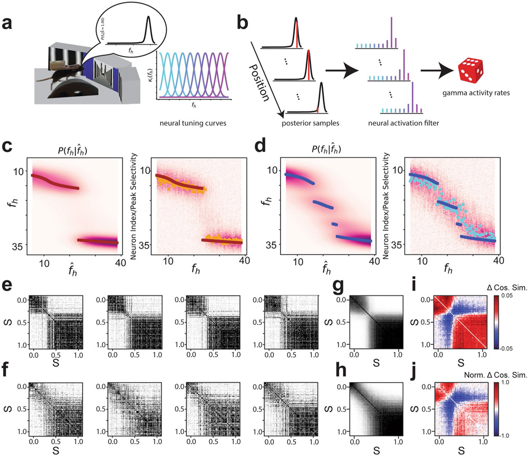
Extended Data Fig. 3 ∣. Remapping patterns for a simulated population designed to stochastically encode the posterior distribution reproduces our recorded remapping patterns.
a, Schematic for model of a ‘neural posterior’. Left: As the animal runs down the track, it tries to infer the identity of the environment it is occupying. The probability of the environment is given by the posterior distribution. Right: We assume that the activity of the neurons we are observing is governed by radial basis function tuning curves for distinct values of the inferred stimulus. b, Process for generating activity. Left: As the animal runs down the track, a process generates several random samples from the posterior distribution. Middle: Each of these samples is filtered through the deterministic neural tuning curves shown in (a). Right: Cellular activity rates are generated by a gamma process with parameters determined by the neural activation. Gamma processes were chosen, as calcium activity rate is a continuous variable. Mean and variance of gamma processes were chosen to be identical so they were more Poisson-like. c, Left: The ideal rare morph posterior distribution as plotted in Fig. 1f (top right) and elsewhere. Right: The activity of a simulated population that encodes samples from the rare morph posterior is shown for different fh values. Each row of the heat map is the activity of a single cell sorted by the fh values for which it has peak selectivity. Each column is the value of fh used to generate a draw from the posterior distribution. Color (white to purple) indicates the average activity of the cell across 1000 draws from the posterior distribution. Yellow points show the index in the population that has the highest average activity rate. Maroon points indicate the ideal rare morph MAP estimates as in left. Note the similarity between the ideal posterior distribution (left) and the activity of the population designed to encode it (right). d, Same as (c) for simulations using the ideal frequent morph posterior distribution. e, Example trial by trial similarity matrices for simulated populations encoding the rare morph posterior. f, Same as (e) for simulated populations encoding the frequent morph posterior. g, Average rare morph trial x trial similarity matrix (n = 1,000 simulations). h, Average frequent morph trial x trial similarity matrix (n = 1,000 simulations). i, Difference in mean trial x trial similarity matrices (rare [g] - frequent [h]). j, Same as (i) but similarity matrices are z-scored prior to averaging (diagonal elements excluded).

