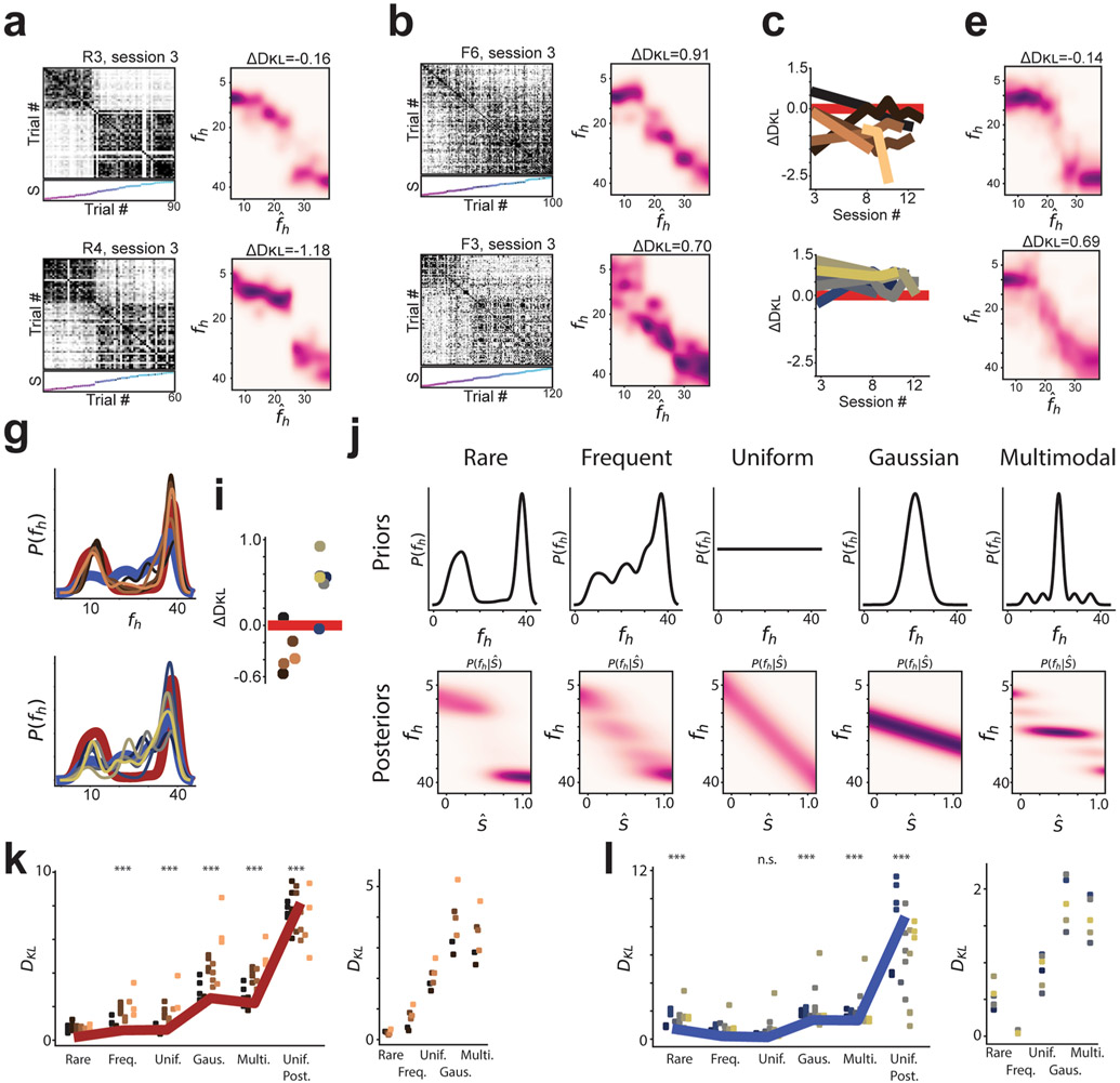
Extended Data Fig. 9 ∣. Session 3 remapping patterns are consistent with later session remapping in the majority of animals, and results are poorly fit by null posterior distributions.
a, Left Column: Trial by trial similarity matrices for session 3 from two rare morph mice (R3-1,973, 90 trials; R4-922 cells, 60 trials). Trials sorted by increasing morph value. Right column: Q estimates for example sessions. b, Same as (a) for example frequent morph sessions (F6, 3,657 neurons, 100 trials; F3, 295 cells, 120 trials). c, ΔDKL for each rare morph mouse plotted as a function of session number. Session 3 data unavailable for R6. d, Same as (c) for frequent morph animals. e, Q estimate for accumulated session 3 data across rare morph mice, f, Same as (e) for frequent morph mice, g-h, Reconstructed prior distributions for rare (g) and frequent (h) morph mice using session 3 data alone. Average rare (maroon) and frequent (blue) morph prior are shown. i, Relative distance of reconstructed priors to ideal priors, ΔDKL, for each mouse (rare mice-left; frequent mice-right). j, Top: Prior distributions for additional models tested for comparison with Q estimates. Bottom: Associated posterior distributions for each prior. We additionally compared Q estimates to a uniform posterior (, where c is a constant). k, Left: Kullback-Leibler divergence (DKL) between each posterior in (j) and the Q estimate. Points are colored by mouse ID. Thick maroon line indicates the across session average. (***) indicate significant differences in DKL with the rare morph DKL values (Wilcoxon signed-rank test, n = 24 sessions; frequent, p = 2.3 × 10⁻⁴; uniform, p = 4.7 × 10⁻⁴; Gaussian, p = 1.8 × 10⁻⁵; multimodal, p = 1.8 × 10⁻⁵; uniform posterior, p = 1.82 × 10⁻⁵). Right: DKL between reconstructed prior and different priors shown in (j). I, Same as (k) for frequent morph sessions. Left: Thick blue line indicates across session average. Wilcoxon signed rank tests compare DKL for the frequent morph condition to DKL for all other posteriors in (j) (Wilcoxon signed-rank test, n = 21 sessions; rare, p = 6.0 × 10⁻⁵; uniform, p = 0.019; Gaussian, p = 6.0 × 10⁻⁵; multimodal, p = 6.0 × 10⁻⁵; uniform posterior, p = 6.0 × 10⁻⁵).

