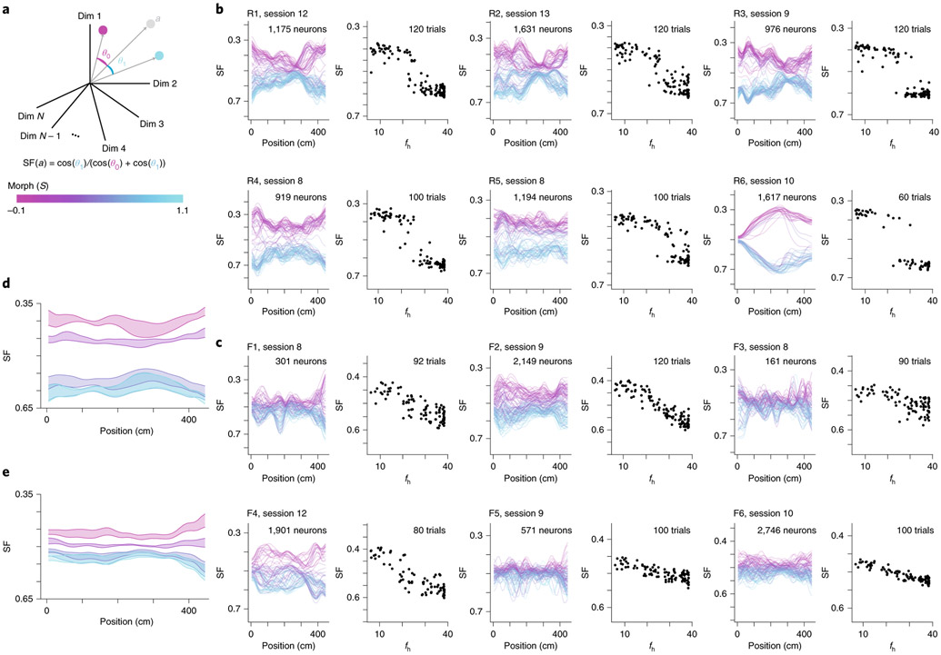
Fig. 4 ∣. CA1 representations show stable discrimination of morph values along the length of the track.

a, Schematic of how the SF is calculated. Each dimension indicates the activity of a single neuron at a single position bin. For the left panels in b and c, only one position bin is included in the calculation at a time. The $\tilde{S}=0$ centroid is calculated by averaging the population vector for all $\tilde{S}=0$ trials (magenta dot). Likewise, the $\tilde{S}=1$ centroid is calculated by averaging the vector for all $\tilde{S}=1$ trials (cyan dot). b, Data for an example session from all mice in the rare morph condition. Left panels show the SF plotted as a function of the position of the animal on the track for each trial in an example rare morph session (for example, mouse R3, session 9; 976 cells, 120 trials). Each line represents a single trial, and the color code indicates the morph value (color bar in a). Right panels show the SF(f_h) plotted (black dots, left vertical axis) as a function of f_h for the same example session shown on the left. Each dot represents a single trial, c, Same as b, but for an example session from all mice in the frequent morph condition. All individual sessions from all are mice shown in Extended Data Figs. 7 and 8. d, Average SF by position plot across rare morph sessions (8–N) and animals (R1–R6). Shaded regions represent across-animal means for binned morph values ($\tilde{S}=0$, 0.25, 0.50, 0.75 and 1.0) ± s.e.m. across mice. Note that the data for morph values 0.75 and 1.0 are nearly overlapping, e, Same as d, but for all frequent morph sessions (8–N, F1–F6 mice, n = 19 sessions). Note that the data for morph values 0.5, 0.75 and 1.0 are partially overlapping.