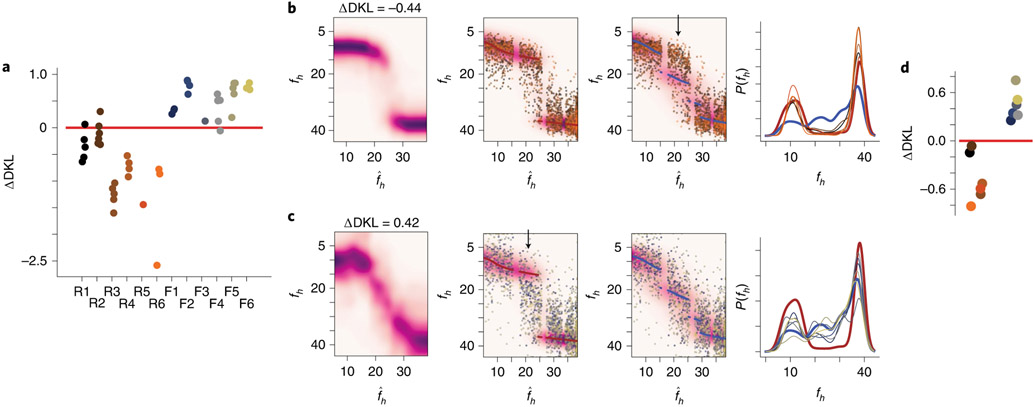
Fig. 6 ∣. Individual animal prior distributions can be recovered solely from remapping patterns.

a, Relative distances of the Q estimates for each session to the ideal rare morph and frequent morph posteriors, ΔD_KL. Each dot represents an individual session. The mouse ID is on the horizontal axis. Jitters were added to the horizontal location for visibility. b, Left: Q estimate achieved by averaging and re-normalizing the across-session Q estimate for each mouse. Middle left: the background heatmap is the ideal rare morph posterior distribution. The maroon scatterplot points are the MAP estimate from this ideal posterior. The remaining points are the linearly transformed SF(f_h) values (as in Fig. 5a, rightmost panel) for every trial and every mouse (n = 2,610 trials). Colors indicate the mouse ID. Middle right: same transformed SF data as in the middle left, but plotted with the ideal frequent morph posterior (heatmap) and MAP estimates (blue scatterplot). The black arrow indicates a mismatch between the transformed SF(f_h) values and the ideal posterior. Right: ideal rare morph prior distribution (maroon), ideal frequent morph prior distribution (blue) and the reconstructed prior for each rare morph mouse (colors indicate mouse the ID). Note that this is the unsupervised recovery of the priors. c, Same as b, but for accumulated data from all mice in the frequent morph group (n = 1,986 trials). d, Relative distances of reconstructed priors (left: rare morph mice; right: frequent morph mice) to either ideal prior, ΔD_KL.