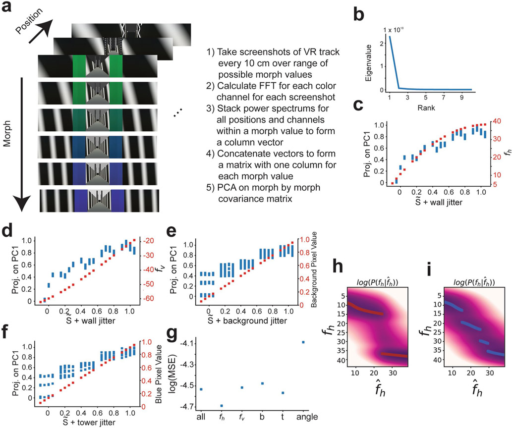
Extended Data Fig. 2 ∣. Across Virtual Reality (VR) scene variance is best predicted by the horizontal component of the frequency of wall cues.

a, Schematic of how across scene covariance was determined. Screenshots of the virtual scene were taken at every 10 cm for the range of possible wall, tower, and background morph parameter settings. Translation invariant representations of these VR scenes were acquired by calculating the two-dimensional Fast Fourier Transform (FFT) of every screenshot on each color channel (RGB). Discarding phase information, we took the power spectrum for each channel and each screenshot. We flattened each of the FFT power spectrums into a column vector. Column vectors for every color channel and every position along the track were concatenated for a given morph parameter setting. This procedure gives one column vector for each morph parameter setting. We then horizontally stacked these column vectors for each morph parameter setting to give a matrix that we used to calculate a morph by morph covariance matrix. We then performed Principal Components Analysis (PCA) on this matrix. b, The eigenvalues of the morph by morph covariance matrix are plotted. c, The projection of each morph parameter setting onto the first principal component (PC1) from (a) plotted as a function of the wall morph value ($\tilde{S}$ + wall jitter)(left vertical axis, blue points). The horizontal component of the frequency of the wall cues, f_h, is also plotted (right vertical axis, red points). d, The projection of each morph parameter setting onto PC1 is plotted as a function of wall morph value (left vertical axis, blue points). The vertical component of the frequency of the wall cues, f_v, is also shown (right vertical axis, red points). e, The projection of each morph parameter setting onto PC1 is plotted as a function of tower morph value ($\tilde{S}$+ tower jitter)(left vertical axis, blue points). The normalized blue color channel pixel value of the towers is also plotted (right vertical axis, red points). The normalized green color channel pixel value of the tower is one minus the blue color channel. f, The projection onto PC1 is plotted as a function of background morph value ($\tilde{S}$+ background jitter). The normalized background color pixel intensity is also plotted (right vertical axis, red points). g, The log of the mean squared error (log(MSE)) of a linear regression to predict the projection of morph parameter settings onto PC1 is plotted for models using different sets of predictors. The ‘all’ model uses f_h, f_v, background pixel value (b), tower blue pixel value (t), and the angle of the wall cues (angle) as predictors of the projection onto PC1. The failure of this model is likely due to the strong correlation among stimulus values. Every other model uses only a single aspect of the stimulus to predict the projection onto PC1. The horizontal component of wall frequency, f_h, is the strongest predictor of the projection onto PC1. h, Ideal rare morph log posterior distribution as plotted Fig. 1f. i. Ideal frequent morph log posterior distribution as plotted Fig. 1f.