Quantitative Techniques and Graphical Representations for Interpreting Results from Alternating Treatment Design

Abstract

Multiple quantitative methods for single-case experimental design data have been applied to multiple-baseline, withdrawal, and reversal designs. The advanced data analytic techniques historically applied to single-case design data are primarily applicable to designs that involve clear sequential phases such as repeated measurement during baseline and treatment phases, but these techniques may not be valid for alternating treatment design (ATD) data where two or more treatments are rapidly alternated. Some recently proposed data analytic techniques applicable to ATD are reviewed. For ATDs with random assignment of condition ordering, the Edgington’s randomization test is one type of inferential statistical technique that can complement descriptive data analytic techniques for comparing data paths and for assessing the consistency of effects across blocks in which different conditions are being compared. In addition, several recently developed graphical representations are presented, alongside the commonly used time series line graph. The quantitative and graphical data analytic techniques are illustrated with two previously published data sets. Apart from discussing the potential advantages provided by each of these data analytic techniques, barriers to applying them are reduced by disseminating open access software to quantify or graph data from ATDs.

Alternating treatment design (ATD) is a single-case experimental design (SCED1), characterized by a rapid and frequent alternation of conditions (Barlow & Hayes, 1979; Kratochwill & Levin, 1980) that can be used to compare two (or more) different treatments, or a control and a treatment condition. An ATD can be understood as a type of “multielement design” (see Hammond et al., 2013; Kennedy, 2005; Riley-Tillman et al., 2020; see Barlow & Hayes, 1979, for a discussion), but it important to mention two potential distinctions. On the one hand, the term “multilelement design” is employed when an ATD is used for test-control pairwise functional analysis methodology (Hagopian et al., 1997; Hall et al., 2020; Hammond et al., 2013; Iwata et al., 1994). On the other hand, a multielement design can be used for assessing contextual variables and ATD for assessing interventions (Ledford et al., 2019). Previous publications on best practices for applying ATD recommend a minimum of five data points per condition, and limiting consecutive repeated exposure to two sessions of any one condition (What Works Clearinghouse, 2020; Wolery al., 2018). The rapid alternation between conditions distinguishes ATDs from other SCEDs, which are characterized by more consecutive repeated measurements for the same condition (Onghena & Edgington, 2005).

In relation to the previously mentioned distinguishing features of ATDs, it is important to adequately identify under what conditions this design is most useful and should be recommended to applied researchers. ATDs are applicable to reversible behaviors (Wolery et al., 2018) that are sensitive to interventions that can be introduced and removed fast, prior to maintenance and generalization phases of treatment analyses. Thus, for nonreversible behaviors, an AB (Michiels & Onghena, 2019), a multiple-baseline and/or a changing-criterion design can be used (Ledford et al., 2019), whereas for reversible behaviors and interventions that require more time to demonstrate a treatment effect (or for an effect to wear off), an ABAB design is typically recommended.

ATD can be useful for applied researchers for several reasons. First, an ATD can be used to compare the efficiency of different interventions (Holcombe et al., 1994), instead of only comparing a baseline to an intervention condition. Second, an ATD enables researchers to perform, in a brief period of time, several attempts to demonstrate whether one condition is superior to the other. This rapid alternation of conditions is useful to reduce the threat of history because it decreases the likelihood that confounding external events occur exactly at the same time as the conditions change (Petursdottir & Carr, 2018). This rapid alternation is also useful to reduce the threat of maturation, which usually entails a gradual process (Petursdottir & Carr, 2018), because the total duration of the ATD study is likely to be shorter when conditions change rapidly and the same condition is not in place for many consecutive measurements. Third, an ATD entailing a random determination of the sequence of conditions further increases the level of internal validity and makes the design equivalent to medical N-of-1 trials, which also entail block randomization and are considered Level-1 empirical evidence for treatment effectiveness for individual cases (Howick et al., 2011). The use of randomization when determining the alternating sequence has been recommended (Barlow & Hayes, 1979; Horner & Odom, 2014; Kazdin, 2011) and is relatively common: Manolov and Onghena (2018) report 51% and Tanious and Onghena (2020) report 59% of the ATD studies use randomization in the design. The fact that randomization is not always used limits the data analysis options available to the investigator. In the following paragraphs, we refer to different options for determining the condition sequence for ATDs. It is important to note that the way in which the sequence is determined affects the number of options available for data analysis.

Among the possibilities for a random determination for condition ordering, a completely randomized design (Onghena & Edgington, 2005) entails that the conditions are randomly alternated without any restriction, but this could lead to problematic sequences such as AAAAABBBBB or AAABBBBBAA. Given that such sequences do not allow for a rapid alternation of conditions, other randomization techniques are more commonly used to select the ordering of conditions. In particular, a “random alternation with no condition repeating until all have been conducted” (Wolery et al., 2018, p. 304) describes block randomization (Ledford, 2018) or a randomized block design (Onghena & Edgington, 2005), in which all conditions are grouped in blocks and the order of conditions within each block is determined at random. For instance, sequences such as AB-BA-BA-AB-BA and BA-AB-BA-BA-AB can be obtained. A randomly determined sequence arising from an ATD with block randomization is equivalent to the N-of-1 trials used in the health sciences (Guyatt et al., 1990; Krone et al., 2020; Nikles & Mitchell, 2015), in which several random-order blocks are referred to as multiple crossovers. Another option is to use “random alternation with no more than two consecutive sessions in a single condition” (Wolery et al., 2018, p. 304). Such an ATD with restricted randomization could lead to a sequence such as ABBABAABAB or AABABBABBA, with the latter being impossible when using block randomization. An alternative procedure for determining the sequence is through counterbalancing (Barlow & Hayes, 1979; Kennedy, 2005), which is especially relevant if there are multiple conditions and participants. Counterbalancing enables different ordering of the conditions to be present for different participants. For instance, the sequence could be ABBABAAB for participant 1 and BAABABBA for participant 2.

Aims and Organization

In the remaining sections of this manuscript, the emphasis is placed on data analysis options for ATD data. In particular, we illustrate the use of several quantitative techniques as complements to (rather than substitutes for) visual analysis. Quantifications are highlighted in relation to the importance of increasing the objectivity of the assessment of intervention effectiveness (Cox & Friedel, 2020; Laraway et al., 2019), reducing difficulties with accurately identifying clear differences between ATD data paths (Kranak et al., 2021), and making ATD results more likely to meet the requirements for including the data in meta-analyses (Onghena et al., 2018). The descriptive quantifications of differences in treatment effects and the inferential techniques (i.e., a randomization test) are applicable to both ATDs with block randomization and restricted randomization. However, the quantifications for assessing the consistency of effects across blocks are only applicable to ATDs with block randomization assignment for the conditions. The analytical options the current manuscript focuses on are scattered across several texts published since 2018. This article is aimed at providing behavior analysts with additional data analytic options, using freely available web-based software.

In the following text, we first discuss visual analysis, several descriptive quantitative techniques, and one inferential statistical technique. Next, we provide potential advantages for the proposed quantifications that complement visual inspection of graphed ATD data. Third, in order to enhance the applicability of the techniques and to make possible the replication of the results presented, we describe several existing software for data analysis options. Finally, we illustrate these quantitative data analytic techniques with two previously published ATD data sets.

Data Analysis Options for Alternating Treatment Design

Visual Analysis

Visual inspection has long been the first choice for investigators (Barlow et al., 2009; Sidman, 1960). The data analysis focuses on the degree to which the data path for one condition is differentiable from (and clearly superior to) the data path for the other condition (Ledford et al., 2019). The data paths are represented by lines connecting sessions within each condition of the ATD. Thus, visual analysis assesses the magnitude and consistency of the separation between conditions (Horner & Odom, 2014), also referred to as differentiation (Riley-Tillman et al., 2020) between the data paths (e.g., whether they cross or not and what is the vertical distance between them). This comparison usually incorporates consistency and level or magnitude of the difference in the dependent variable across the treatment conditions (Ledford et al., 2019).

Descriptive Data Analytic Techniques

The main strengths and limitations of the descriptive data analytic techniques reviewed are presented in Table 1. Examples of their use are provided in the section entitled “Illustrations and Comparison of the Results,” including a graphical representation of most of these techniques. In Table 1, we also refer to the particular figure that represents an application of a technique.

Table 1.

Summary of the main features of several data analytic techniques applicable to alternating treatments designs

Data analytical technique	Data aspect quantified	Strengths	Limitations	Calculation	Example
Visual structured criterion (VSC)	Superiority of one condition over the other, by means of comparing data paths.	Corresponds directly to the visual inspection of the data, which focuses on the differentiation or separation between data paths.	The comparison is only ordinal (i.e., one condition is either superior, equal or inferior to the other) without quantifying the distance. The outcome is binary: meets or does not meet the criterion for superiority. The comparison excludes the first and last measurements for which only one of the data paths is present.	For each measurement occasion, a comparison is performed between the data paths for the two conditions. The number of comparisons for which one condition is superior is tallied. This tally is compared to a predefined criterion developed by the authors via a simulation study.	Figure 7 can be used, focusing on the number of green arrows out of the total number of comparisons.
Average difference using actual and linearly interpolated values (ALIV)	Quantifies the distance between the data paths (i.e., the line connecting the points from one condition is compared to the line connecting the points from the other condition).	Corresponds directly to the visual inspection of the data, which focuses on the differentiation or separation between data paths.	Includes interpolated values, which are assumed to represent the value that would have been obtained under the condition not taking place. The comparison excludes the first and last measurements for which only one of the data paths is present.	For each measurement occasion, a measurement obtained in one condition is compared to the measurement interpolated (according to the data path) for the other condition. An average difference is computed for all measurement occasions.	Figure 7
Average difference between successive observations (ADISO)	Quantifies the differences between successive observations belonging to different conditions.	Uses only actually obtained measurements, without modeling (interpolation, trend lines, reducing the measurements to a single average). Expressed in the same measurement units as the target behavior.	For certain alternating sequences (i.e., the ones that cannot be obtained when using block randomization), the use of ADISO requires deciding how to segment the alternating sequence (e.g., AABBAABAB can be divided as AABB-AAB-AB or AAB-BA-AB-AB).	The measurement(s) from one condition in its first application are compared to the adjacent measurement(s) in the other condition in its first application, and so forth for the entire alternation sequence. An average difference is computed for all repetitions of the alternation between the two conditions.	Figure 8
Visual aid and objective rule (VAIOR)	Establishes a reference, on the basis of baseline trend and variability, to which to compare the intervention phase data in order to assess whether the degree of superiority is sufficient.	Considers both baseline trend and baseline variability, when representing a reference for assessing the intervention phase data.	A straight line may not represent sufficiently well the data, especially if estimated from few baseline data points.	Fits and projects baseline trend. Quantifies baseline data variability and projects a variability band. Identifies whether the intervention improves sufficiently these projections.	Figures 4 and 6
Consistency of effects across blocks (CEAB)	Quantifies the degree of lack of consistency of effects across blocks, expressed as a percentage of variance (from the whole variability in the measurements).	Uses the well-known analysis of variance for partitioning variance due to the intervention effect, due to the difference across blocks, and due to the interaction of the blocks and the intervention.	Only applicable to ATDs with block randomization.	Quantifies, via analysis of variance, the proportion of variability in the measurements of the dependent variable that is not explained either by the intervention or the blocks (i.e., the interaction of these two factors).	Figure 2
Consistency of data features in similar conditions, quantified as mean absolute percentage error for similar conditions (MAPESIM)	Quantifies the consistency in the measurements for the same condition. Performs the quantifications separately for each condition	Easily represented graphically via the modified Brinley plot.	Most easily applied to ATDs with block randomization in order to represent each block with a dot in the modified Brinley plot.	Represents the values of each block in a two-dimensional space in which each dimension is one of the conditions. Quantifies the vertical and horizontal distances between each dot and the averages per condition. Expresses the average of these distances in relation to the average value for the condition.	Figure 3
Consistency of effects quantified as mean absolute percentage error for different conditions (MAPEDIFF)	Quantifies the consistency of the difference between adjacent raw measurements belonging to different conditions.	Easily represented graphically via the modified Brinley plot.	Most easily applied to ATDs with block randomization in order to represent each block with a dot in the modified Brinley plot.	Represents the values of each block in a two-dimensional space in which each dimension is one of the conditions. Quantify the vertical distance between each dot and diagonal line representing the mean difference between conditions. Expresses the average of these distances in relation to the mean difference.	Figure 9

Comparing Data Paths

Quantifying the difference between the data paths entails using observed behavior via direct measurement and linearly interpolated values. The linearly interpolated values are the specific locations within a data path for one condition; they lie between session data points from that condition. The interpolated data points represent the value that hypothetically would have been obtained for a given condition if it had taken place on a given measurement occasion; however, in the ATD, the alternative treatment condition is imposed instead.

One approach to comparing two or more data paths is to use the visual structured criterion (VSC; Lanovaz et al., 2019). The comparison is performed ordinally, that is, considering only whether one condition is superior to the other; it does not measure the degree of superiority (unlike the quantification described in the following paragraph). In particular, the VSC first quantifies the number of comparisons (measurement sessions) for which one condition is superior. Afterwards, the VSC compares this quantity to the cut-off points empirically derived by Lanovaz et al. (2019) for detecting superiority greater than one expected by chance.

A comparison involving actual and linearly interpolated values (abbreviated as ALIV, Manolov & Onghena, 2018) assesses the magnitude of effect, by focusing on the average distance between the data paths. Complementary to the visual structured criterion, ALIV quantifies the magnitude of the separation between data paths.

Assessment of Level and Trend

Comparing data paths is common in visual analysis of graphed SCED data, and in many ways relies on implicit use of interpolated values between sessions for each data path. In addition to visual comparison, a quantification using only the obtained (observed) measurements may be preferable to a quantification using the interpolated values from the ALIV. A possible quantification using only observed values is the “average difference between successive observations” (ADISO; Manolov & Onghena, 2018). As suggested by Ledford et al. (2019), measurements from one condition are compared to adjacent measurements of the other condition. The calculations focus on level, whereas potential distinct trends are quantified via increasing or decreasing differences between adjacent values. For an ATD with block randomization of condition ordering, it is straightforward to perform the comparisons within blocks. However, a substantial limitation arises when ADISO is used for ATD data with restricted randomization because the analyst would have to decide exactly how to segment the alternation sequence (i.e., which comparisons to perform). With different segmentations, the quantification of the difference between conditions can lead to different results. The recommendation is to segment the sequence in such a way that it allows for the maximum number of possible comparisons (e.g., segment AABBABBAABBA as AABB-AB-BA-AB-BA and not as AAB-BA-BBAA-BBA). In cases where different segmentations lead to the same number of comparisons (e.g., BAABAABABABB can be segmented as BAA-BA-AB-AB-ABB and BA-AB-AAB-AB-ABB), a sensitivity analysis comparing the results across different segmentations is warranted.

Taking into Account the Variability within Conditions

In ATD research, the measures of variability within a condition commonly reported are the (1) range and (2) standard deviation (Manolov & Onghena, 2018). Beyond reporting these values, the “visual aid and objective rule” (VAIOR, Manolov & Vannest, 2019) also includes the degree of variability within conditions. VAIOR assesses whether the data from one condition are superior to the data from the other condition, with the latter being summarized by a trend line and a variability band. The trend line is fitted by applying the Theil-Sen method (Vannest et al., 2012) to the data obtained in one condition (usually the baseline condition or another reference condition). The Theil-Sen method is a robust (i.e., resistant to outliers) technique based on finding the median of the slopes of all possible trend lines connecting all values pairwise. The variability band is constructed on the basis of the median absolute deviations from the median, which is a measure of scatter that is also resistant to outliers. The assessment in VAIOR focuses on whether the data from a given condition exceed the variability band. Similar to the visual structured criterion, a dichotomous decision is reached regarding whether there is sufficient evidence for the superiority of one condition over another with the degree of variability within each condition affecting this determination.

Consistency of Effects when Comparing Conditions

When analyzing SCED data, the consistency of the data within the same condition and the consistency of effects are two crucial aspects for establishing a functional relation between the independent variable, which causes the observed change (if any) on the dependent variable (Lane et al., 2017; Maggin et al., 2018). Two different approaches can be used for quantifying the consistency of effects for data obtained following an ATD with block randomization. The first is called “consistency of effects across blocks” (CEAB), is based on variance partitioning (Manolov et al., 2020): the total variance is divided into variance explained by the intervention effect, variance attributed to differences between blocks, and residual or interaction variance. The total variance is the sum of the squared deviations between any value and the mean of all values. The explained variance basically reflects the squared differences between the mean in each condition and the mean of all values, regardless of the condition in which they were obtained. The variance attributed to the blocks reflects the squared differences between the mean of the values from each block (mixing both conditions being compared) and the mean of all values. The variance represents the lack of consistency of the effect across blocks because the difference between conditions is larger in some blocks than others. The smaller the residual or interaction variability, the more consistent the effect was across blocks. In the context of this data analytic technique, several graphical representations are also suggested to facilitate interpreting the CEAB (Manolov et al., 2020), as shown in the section entitled “Illustrations and Comparison of the Results.”

Another approach is based on a graphical representation called the modified Brinley plot (Blampied, 2017) in which the measurements in one condition are plotted (on the Y-axis) against the measurements in the other condition (on the X-axis). A single data point represents the block. For designs that have phases (e.g., a multiple-baseline design or an ABAB design), each point represents the mean of a phase for a condition, with baseline means represented on the X-axis and adjacent intervention phase means on the Y-axis. A diagonal line (slope = 1, intercept = 0) shows the absence of difference or the equality between conditions. If all points are above the diagonal line, there is consistent superiority of treatment over baseline (assuming a high score represents improvement). If all points are below the diagonal then the treatment made behavior worse. The consistency in the magnitude of the effect across blocks is assessed in relation to the degree to which the points are close to a parallel diagonal line marking the average difference between conditions. If the slope is not equal to 1.0, then the interpretation is a bit more complex but quite revealing. If, for example, the treatment works best when baseline values are low, then data points on the left end of the graph will be farther above the baseline than points on the right end.

The calculation is actually a mean absolute percentage error, computed when comparing different conditions, which is why this data analytical technique is abbreviated MAPEDIFF (Manolov & Tanious, 2020). Thus, the modified Brinley plot can be used to represent visually the outcome of the specific comparisons performed between measurements in an ATD with block randomization) or between phases in a multiple-baseline or an ABAB design. It also enables checking whether the direction of the difference is consistently in favor of one of the conditions, whether this difference is of sufficient magnitude for all comparisons (in case a meaningful cut-off point is available), whether treatment efficacy depends on baseline levels, and whether this difference is consistent across all comparisons.

In both cases, the consistency of effects can be conceptualized as the degree to which variability of the effects observed in the different blocks are comparable to the average of these effects across blocks. Nonetheless, we prefer to separate the assessment of variability (usually assessed within each condition separately, before exploring whether there is a difference in variability across conditions), from the assessment of consistency of effects (which necessarily entails a comparison across conditions). These separate assessments are well-aligned with the recommendations for performing visual analysis (Lane et al., 2017; Ledford et al., 2019; Maggin et al., 2018).

Inferential Data Analytical Techniques

In the following section we refer to randomization tests as an inferential technique based on a stochastic element in the design (i.e., the use of randomization for determining the alternation sequence for conditions). In fact, randomization tests are the historically first statistical option proposed for ATD (Edgington, 1967; Kratochwill & Levin, 1980) and several studies using ATD have applied this analytical option (Weaver & Lloyd, 2019). However, despite the frequent use of randomization of condition assignment, the application of randomization tests are not yet commonly used with SCEDs (Manolov & Onghena, 2018). The aim of the current section is to justify and encourage both the use of randomization of condition presentation and the employment of randomization tests as an inferential analytical tool, as well as to describe their main features. Other inferential techniques, based on random sampling, are not discussed here. The interested reader is referred to regression-based procedures for model-based inference (Onghena, 2020). In particular, these techniques allow modeling the average level of the measurements in each condition and, if desired, the trends. The readings suggested for regression-based options in the SCED context are Moeyaert et al. (2014), Shadish et al. (2013), and Solmi et al. (2014), whereas for options in the context of N-of-1 trials Krone et al. (2020) and Zucker et al. (2010) can be consulted.

What is Gained by Using Randomization of Condition Ordering

Randomization can address threats to internal validity and increase the scientific credibility of the results of a study, including SCED studies (Edgington, 1996; Kratochwill & Levin, 2010; Tate et al., 2013). For ATDs, alternating the sequence randomly makes it less likely that external events are systematically associated with the exact moments in which conditions change. Randomization, along with counterbalancing, has also been suggested for decreasing condition sequencing effects, i.e., the possibility that one condition consistently precedes the other condition (Horner & Odom, 2014; Kennedy, 2005). The usefulness of randomization for addressing threats to internal validity is likely the reason for original introduction of ATDs as discussed by Barlow and Hayes (1979).

The inclusion of randomization of condition ordering in the design also allows the investigator to use a specific analytical technique called randomization tests (Edgington, 1967, 1975). Randomization tests are applicable across different kinds of SCEDs (Craig & Fisher, 2019; Heyvaert & Onghena, 2014; Kratochwill & Levin, 2010), as long as there is randomization in the design, such as the random assignment of conditions to measurement occasions (Edgington, 1980; Levin et al., 2019). Randomization tests are also flexible in the selection of a test statistic according to the type of effect expected (Heyvaert & Onghena, 2014). In particular, the test statistic can be defined according to whether the effect is expected to be a change in level or in slope (Levin et al., 2020), and whether the change is expected to be immediate or delayed (Levin et al., 2017; Michiels & Onghena, 2019). The test statistic is just the computation of a specific measure of the difference between conditions that is of interest to the researcher for which a p-value will be obtained. Owing to the presence of randomization in condition ordering, there is no need to refer to any theoretical sampling distribution that would require random sampling. The test statistic is usually the mean difference actually obtained, due to its frequent use as a summary measure in ATD (Manolov & Onghena, 2018). Any aspect of the observed data (e.g., level, trend, overlap2) or any effect size or quantification (e.g., ALIV; Manolov, 2019) can be used as a test statistic. To conduct the analysis, the test statistic is computed for the actual (obtained) alternation sequence (for instance, ABBAAB). Then the same test statistic is computed for all possible alternation sequences. In particular, the measurements obtained (e.g., 6, 8, 9, 7, 5, 7) maintain their order as they cannot be placed elsewhere due to the likely presence of autocorrelation in the data (Shadish & Sullivan, 2011). What changes in each possible alternation sequence, from which the actual alternation sequence was selected at random, are the labels, which denote the treatment conditions. Thus, when constructing the randomization distribution, other possible orderings/labels such ABABAB and ABABBA are assigned to each measurement in its original sequence (6, 8, 9, 7, 5, 7) and the test statistic is computed according to these labels. The randomization distribution is constructed by computing the test statistic for all possible alternation sequences, whose number is 2^k when there are k blocks or pairs of conditions and for each block a random selection is performed regarding which condition is first and which section (Onghena & Edgington, 2005). The actually obtained test statistic is compared to the test statistics computed for all possible alternation sequences under the randomization scheme (these are called “pseudostatistics,” because they are computed for alternating sequences that did not actually take place, but are ones that could possibly occur). If an increase in the target behavior is desired, the p-value is the proportion of pseudostatistics as large as or larger than the actual test statistic. As an alternative, if a decrease is the aim of the intervention, the p-value is the proportion of pseudostatistics as small as or smaller than the actual test statistic.

As an additional strength, although their use requires random ordering of conditions for each participant, randomization tests are free from the assumptions of random sampling of participants from a population, normality or independence of the data (Dugard et al., 2012; Edgington & Onghena, 2007). This is important, because in the SCED context it cannot be assumed that either the individual or their behavior were sampled at random. Moreover, the data are autocorrelated and not necessarily normally distributed (Pustejovsky et al., 2019; Shadish & Sullivan, 2011; Solomon, 2014). Finally, when using a randomization test, missing data can be handled effectively in a straightforward way by randomizing a missing-data marker, as if it were just another observed value, when obtaining the value of the test statistic for all possible random assignments (De et al., 2020). There is no specific limitation that the use of randomization of condition ordering entails because it is also possible to combine randomization and counterbalancing (e.g., see Edgington & Onghena, 2007, ch. 6). This could occur, for instance, when determining the sequence at random for participant 1 (e.g., ABABBAAB) and counterbalancing for participant 2 (i.e., BABAABBA).

Interpreting the p-Value

The null hypothesis is that there is no effect of the intervention and thus the measurements obtained would have been the same under any of the possible randomizations (Jacobs, 2019), and in the ATD case, under any of the possible random sequences. The p-value quantifies the probability of obtaining a difference between conditions as large as, or larger than, the actually observed difference, conditional on there being no difference between the conditions. A small p-value entails that the difference observed is unlikely if the null hypothesis is true. Hence, either we observed an unlikely event or it is not true that the intervention is ineffective. If we don’t believe in unlikely events then our conclusion is tentatively that the intervention is effective, but a statistically significant result does not show the actual probability that the intervention is superior to another treatment or baseline.

In addition, it should be noted that p-values should not be interpreted in isolation. Other analytical methods, such as visual analysis and clinical significance measures, as well as assessment of social validity should be considered as well. We do not suggest that a p-value is the only way for tentatively inferring a substantial treatment effect, because the assessment of the presence of a functional relation is usually performed via visual analysis of graphed data (Maggin et al., 2018), especially in terms of the consistency of the effects (Ledford et al., 2019). However, the p-value based on the presence of randomization in the design is an objective quantification, which is valid thanks to the use of the randomization of condition ordering as it was actually implemented during the study.

Assessing Intervention Effectiveness: Beyond p-Values

A randomization test is not to be applied arbitrarily (Gigerenzer, 2004), nor is it free of interpretation from the researcher (see Perone, 1999). In fact, the researcher chooses a priori the method for choosing the condition ordering at random that is the most reasonable (e.g., block randomization vs. restricted randomization; Manolov, 2019) and which test statistic to use according to the expected effects (change in level or change in trend, immediate or delayed), in relation to the six data aspects emphasized by Kratochwill et al. (2013). Moreover, the researcher is encouraged to use other data analytic outcomes besides the p-value because other sources of data analysis are not discarded or disregarded when interpreting a p-value. In terms of inferential quantifications, confidence intervals are important for informing about the precision of estimates (Wilkinson & The Task Force on Statistical Inference, 1999) and they can be constructed based on randomization test inversion (Michiels et al., 2017). The visual representation of the data should always be inspected, and the individual values can be analyzed. The researchers can, and must, still seek the possible causes of specific outlier measurements according to their knowledge about the client, the context, and the target behavior. Finally, maintenance, generalization, and any subjective opinion expressed by the client or significant others can be considered, along with normative data (if available), to assess the social validity of the results (Horner et al., 2005; Kazdin, 1977).

The Need for Quantifications Complementing Visual Analysis

Visual and Quantitative Analyses should be Used in Conjunction

The quantifications illustrated are not suggested as replacements for the visual inspection of graphed data. They should rather be understood as complementary. Such complements are necessary for several reasons. First, visual and quantitative analyses can achieve different goals. Visual analysis is used to shape an inductive and dynamic approach to identifying the factors controlling the target behavior (Johnson & Cook, 2019; Ledford et al., 2019), or to conduct response-guided experimentation (Ferron et al., 2017). For such purposes, visual analysis enables the researcher to maintain in close contact with the data (Fahmie & Hanley, 2008; Perone, 1999). Quantifications used for a summative purpose can complement this by providing objective and easily communicable results that can be aggregated across participants, avoiding subjectivity and potential confirmation bias in visual analysis (Laraway et al., 2019). Such quantification facilitates the analysis of multiple data sets, making it easier than inspecting each one of them separately (Kranak et al., 2021). In addition, quantifications can be used to integrate the results across studies via meta-analysis (Jenson et al., 2007; Onghena et al., 2018), which is important considering the need for examining the external validity of treatment results. The complementarity between visual and quantitative analyses can be illustrated by data analytic techniques such as ALIV (Manolov & Onghena, 2018), which was developed to quantify exactly the same aspect that is visually evaluated: the degree of separation between data paths. It is possible that a separation or differentiation be of such size that it is easy to identify via visual inspection (Perone, 1999), but a quantification can still be useful for communicating and aggregating the results via meta-analysis of SCED data.

Quantifications Commonly Accompany Visual Analysis

When presenting visual analysis, it is common to refer to visual aids (e.g., trend lines, which are based on quantitative methods) and descriptive quantifications, such as means and overlap indices (Lane & Gast, 2014; Ninci, 2019). In addition, probabilities (such as the ones arising from a null hypothesis test) have also been suggested as tools for aiding visual analysts: see the dual criteria (Fisher et al., 2003), which are commonly recommended and tested in the context of visual analysis (Falligant et al., 2020; Lanovaz et al., 2017; Wolfe et al., 2018).

Why Quantifications Are Useful

Quantifications can help mitigate some of the potential problems associated with visual inspection, such as insufficient interrater agreement (Ninci et al., 2015) or the fact that the graphical features of the plot can affect the result of the visual inspection (Dart & Radley, 2017; Kinney, 2020; Radley et al., 2018). A quantitative analysis requires several decisions to be made which leads to “researcher degrees of freedom” (Hantula, 2019; Simmons et al., 2011), potentially affecting the results through the decisions that were made. However, once an appropriate specific quantitative method is chosen, it yields the same result regardless of how the data are graphed.

Some of the quantifications illustrated in this article (i.e., Manolov et al., 2020; Manolov & Tanious, 2020) refer to an issue that is critical for SCEDs: replication (Kennedy, 2005; Sidman, 1960; Wolery et al., 2010; see also the special issue of Perspectives on Behavior Science on the “replication crisis”: Hantula, 2019) and the consistency of results across replications (Ledford, 2018; Maggin et al., 2018). Considering the fact that p-values in the classical null hypothesis significance testing approach do not provide information about the replicability of an effect (Branch, 2014; Killeen, 2005), we consider that it is important to emphasize quantifications that emphasize the consistency of effects across replications.

Some Quantifications that are Easy to Understand and to Use

Applied researchers are likely to be more familiar with visual analysis and prefer avoiding the steep learning curve required for specialized skills such as advanced statistical analysis. However, most of the quantifications described in the current text are straightforward and intuitive. For instance, ALIV is simply a quantification of the distance between data paths, whereas ADISO is a quantification of the average difference between successive measurements. Likewise, a randomization test entails the calculation of a test statistic (e.g., mean difference between conditions) for the actual alternation sequence as compared with all possible alternation sequences that could have been obtained according to the randomization scheme. There is no need to assume hypothetical sampling distribution with normal distribution of data points. Simple quantifications, like the ones illustrated here, are more likely to be used by applied researchers3 who are typically more familiar with visual inspection of graphically depicted data. Moreover, the quantifications illustrated here are implemented in intuitive and user friendly software that is available for free (e.g., https://tamalkd.shinyapps.io/scda/ and https://manolov.shinyapps.io/ATDesign/).

Open Access Software for Data Analysis

List of Software

The current section provides a list of software that can be used when analyzing ATD data. All software listed, except for the Microsoft Excel macro for randomization tests (https://ex-prt.weebly.com/; Gafurov & Levin, 2020), are user-friendly and freely available websites that do not require that the user has any specific program installed.

• Choosing an alternation sequence at random (i.e., designing the study) and performing a randomization tests for data analysis (Heyvaert & Onghena, 2014; Levin et al., 2012; Onghena & Edgington, 1994, 2005): https://tamalkd.shinyapps.io/scda and https://ex-prt.weebly.com/.

• Comparing data paths via ALIV (Manolov & Onghena, 2018; with the possibility of obtaining a p-value for ALIV on the basis of randomization test, Manolov, 2019) and also as a basis for the visual structured criterion (Lanovaz et al., 2019): https://manolov.shinyapps.io/ATDesign.

• Comparing adjacent data points using ADISO (Manolov & Onghena, 2018): https://manolov.shinyapps.io/ATDesign.

• Visual aid and objective rule (VAIOR; Manolov & Vannest, 2019) for complementing visual analysis, using Theil-Sen trend and a variability band: https://manolov.shinyapps.io/TrendMAD.

• Assessment of consistency on the basis of variance partitioning (Manolov et al., 2020): https://manolov.shinyapps.io/ConsistencyRBD.

• Assessment of consistency in relation to the modified Brinley plot—MAPESIM and MAPEDIFF (Manolov & Tanious, 2020): https://manolov.shinyapps.io/Brinley.

Data Files to Use

The structure of the data file that is required is the same for several instances of software: (1) the randomization test via https://tamalkd.shinyapps.io/scda; (2) for applying the comparison involving actual and linearly interpolated values (ALIV) and the ADISO (Manolov & Onghena, 2018: https://manolov.shinyapps.io/ATDesign); and (3) VAIOR (Manolov & Vannest, 2019: https://manolov.shinyapps.io/TrendMAD). In particular, a simple text file (.txt extension, from Notepad) is required with two columns, separated either by a tab or a comma. One column must contain the header “condition” and it include on each row the letters A and B, marking the condition. The other column should be labeled “score” and it includes the values obtained at each measurement occasion. One data file is required for each alternation sequence (i.e., for each participant). For ADISO, in order to specify where each block ends (i.e., how to split the alternation sequence in blocks), an additional data file is required. A text file with a single line with the last measurement occasion for each block is required—each number separated by commas. For instance, for a design with seven blocks of two conditions, the additional file will contain the following text: 2, 4, 6, 8, 10, 12, 14. This is the specific set of points in which each block ends for a sequence with seven blocks: it is valid not only for the current data, but also for any other sequence that entails seven blocks. Complementary to this, if there are five blocks, the sequence will be 2, 4, 6, 8, 10 and if there are 20 blocks, the sequence will be 2, 4, 6, 8, 10, 12, 14, 16, 18, 20.

For the assessment of consistency via variance partitioning (https://manolov.shinyapps.io/ConsistencyRBD) and the quantifications related to the modified Brinley plot (https://manolov.shinyapps.io/Brinley), a different kind of data file is used. There is a column called “Tier,” which contains only the value 1, given that a single ATD sequence is to be represented (i.e., a single individual)4 and repeated as many time as there are measurements. A second column is called “Id” and it marks the block, repeating twice each consecutive value (e.g., 1, 1, 2, 2, 3, 3, if there are three blocks). The third column is called “Time” and it contains the values making the measurement occasions (1, 2, up to the number of measurements). A fourth column is called “Score” and contains the measurements. A fifth and final column is called “Phase” and contains the values 0 and 1 for conditions A and B, respectively.

In the Open Science Framework Project (https://osf.io/ks4p2) we have included the data for the illustrations, organized as previously described. The data are available in two Microsoft Excel files and to use them it is only necessary to copy the data from each worksheet and paste it into a new text (Notepad) file. The pasting creates a file separated by tabs.

Use of the Software

The websites use point-and-click menus for loading the text files with the data and for obtaining the results. It is possible to modify the default display of the graphical representations by adding visual aids (for https://tamalkd.shinyapps.io/scda) and by changing the minimum and maximum value of the Y-axis and the size of the plot (for the remaining websites from the list). The tabs within each website and the options to be chosen include self-explanatory descriptions.

Illustrations and Comparison of the Results

Selection of Published Data for the Illustrations

Two studies were selected for three reasons: (1) the studies describe procedures consistent with block randomization for the ATD; (2) the studies represent a variety of data patterns—some show clear differences (i.e., completely differentiated data paths that do not cross) and others show more subtle differences (i.e., data paths crossing to different degrees); and (3) the studies were selected to include a variety of data analysis techniques (Fletcher et al., 2010, use visual analysis with means and number of sessions to achieving a criterion, whereas Sjolie et al., 2016, use Cohen’s d and a randomization test).

Only a selection of all possible results from all the data analysis procedures described previously in the manuscript is presented here. Results applying all these previously mentioned quantitative techniques, applied to each of the two data sets, can be obtained from the previously mentioned websites, using the data files from the Open Science Framework Project (https://osf.io/ks4p2). The assessment of presence, magnitude, and consistency of effect is summarized in Table 2.

Table 2.

Quantifications obtained for the data in the three illustrations. For the comparison involving actual and linearly interpolated values (ALIV) and the average difference between successive observations (ADISO), the calculation performed is A minus B. The ADISO superiority percentage refers to the superiority of B over A, except for Retention for Participant 1008 (superiority of A over B).

Study	Fletcher et al. (2010)			Sjolie et al. (2016)
Participant	Ashley	Robert	Ken	Acquisition for 1003	Retention for 1008
VSC	Met	Met	Met	Not met	Not met
VAIOR criterion	Met	Met	Met	Not met	Not met
ADISO	-56.15	-60.00	-75.71	-13.07	5.00
ADISO superiority	100.00%	90.91%	100.00%	85.71%	42.86%
ALIV	-52.50	-62.00	-76.67	-14.96	8.17
ALIV p-value	<.01	<.01	<.01	0.047	0.82
CEAB	88.89%	90.65%	99.13%	71.00%	61.42%
MAPE-A	42.14%	43.64%	42.86%	43.37%	68.40%
MAPE-B	11.38%	9.72%	6.40%	32.57%	30.24%
MAPE-DIFF	30.35%	21.21%	8.09%	97.55%	342.08%

CEAB consistency of effects across blocks, MAPE mean absolute percentage error (A denotes condition A, B denotes condition B, DIFF denotes the effect or difference between conditions), VAIOR visual aid and objective rule, VSC visual structured criterion, NA calculation not available for the data set

ATD Data Reanalyzed

In Fletcher et al. (2010), a comparison was performed between TOUCHMATH, a multisensory mathematics program and a number line, for three middle-school students (Ashley, Robert, and Ken) with moderate and multiple disabilities in the context of solving single-digit mathematics problems. The data for the comparison phase in which the two interventions are alternated are presented in Fig. 1.

Fig. 1.

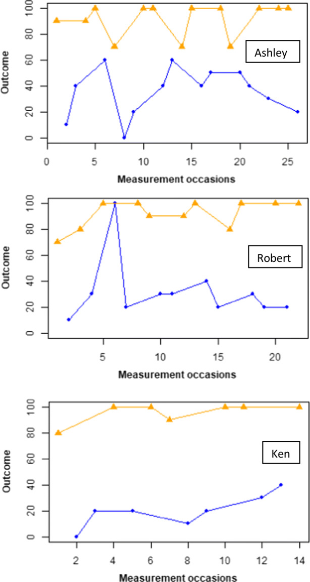
Data gathered by Fletcher et al. (2010) for Ashley (upper panel), Robert (middle panel), and Ken (lower panel). Condition A (number line): blue. Condition B (touch points): yellow. Plots created via https://manolov.shinyapps.io/ConsistencyRBD/

According to Fletcher et al. (2010, p. 454), all students

showed significant improvements using the ‘touch points’ method compared to the number line strategy to solve. . . . During the baseline phase, the students averaged 4% of the single-digit mathematics problems accurately, however, while in the ‘touch points’ phase the students averaged 92% of the problems correctly, compared to only 30% while using the number line strategy.

The authors also mention that each participant reached the criterion of 90% accuracy for three consecutive sessions faster for the touch points program.

Figure 2 represents the differences for each pair of conditions within a block. The closer that the dots are to the red horizontal line, the more similar the differences between conditions in each block. Thus, the differences are most similar (i.e., most consistent) for Ken and more variable (i.e., least consistent) for Ashley. In particular, for Ken, most differences are exactly the same, except for the last two. For Robert, all differences are similar except one 0 difference. For Ashley, there is greater variability.

Fig. 2.

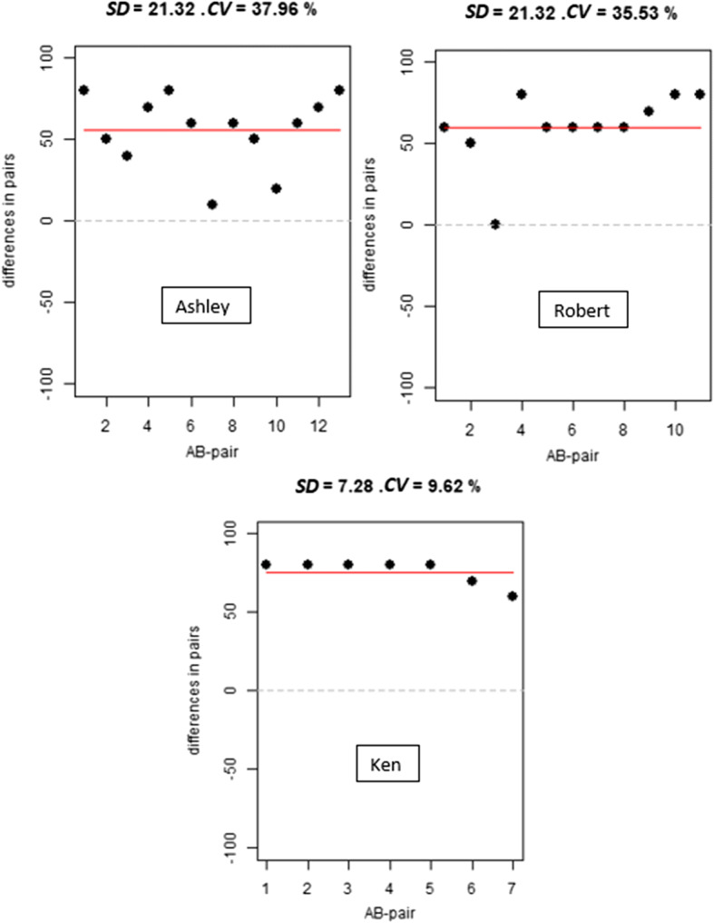
Differences between conditions for each block, for the Fletcher et al. (2010) data for Ashley (upper panel), Robert (middle panel), and Ken (lower panel). The red horizontal line is the mean difference for each participant. The vertical distance between the dots and the red horizontal line visualizes the consistency of the difference between conditions across blocks. Plots created via https://manolov.shinyapps.io/ConsistencyRBD/, as presented by Manolov et al. (2020) in the context of the development of CEAB

In order to further study the results for Ashley, we quantify the degree of consistency for each condition in Fig. 3. This figure represents a modified Brinley plot, constructed as described in Blampied (2017) with the additional graphical aids described Manolov and Tanious (2020). In particular, for ATDs, the coordinates of each data point are defined by a condition A value (X-axis) and the corresponding condition B value (Y-axis) from the same block of the ATD. Both the left and the right panel of Fig. 3 include the same data and thus the same configuration of data points. The left panel focuses on the condition A measurements, represented in the X-axis, and it represents the distance between each condition A value and the condition A mean via the horizontal dashed lines. In complementary fashion, the right panel focuses on the condition B measurements, represented in the Y-axis, and it represents the distance between each condition B value and the condition B mean via the vertical dashed lines. MAE, standing for mean absolute error (also called “mean absolute deviation”) is the average of these horizontal (left panel) or vertical (right panel) distances. Therefore, the longer these horizontal or vertical lines, the larger the value of MAE (mean absolute error) and, thus, the lower the consistency within each condition.

Fig. 3.

Consistency of data points for participant Ashley from the Fletcher et al. (2010) study. The left panel illustrates the consistency in Condition A (number line): the greater the horizontal distance between the points and the vertical line representing the condition A mean, the lower the consistency. The right panel illustrates the consistency in Condition B (touch points): the greater the vertical distance between the points and the horizontal line representing the condition B mean, the lower the consistency. Plots created via https://manolov.shinyapps.io/Brinley/, as part of the MAPESIM quantification (Manolov & Tanious, 2020)

In absolute terms (here, accuracy as a percentage), the MAE from the average level is similar for both conditions. MAE is equal to 14.91 for condition A (number line) and 10.41 for condition B (touch points). However, in relative terms (i.e., the quantification called MAPESIM [mean absolute percentage error for similar conditions]), this variability represents 42% of the mean for condition A (which is equal to 35.38 and thus 14.19/35.38 = 42.14%) and only 11% of the mean for condition B (which is equal to 91.54 and thus 10.41/91.54 = 11.38%), indicating greater consistency for the latter. This is an additional result that can be used for justifying the conclusion of difference between conditions for Ashley. Given that the data paths for Ashley do not cross, the greater variability in condition A can be detected from visual inspection, and MAPESIM serves as a quantitative complement.

Finally, given the greater variability of values in condition A (number line), we checked for evidence regarding whether the improvement observed in condition B (touch points), is sufficient. In Fig. 4, we apply VAIOR (Manolov & Vannest, 2019) to Ashley’s data. Despite the variability, there is no upward or downward overall trend in Condition A. A total of 46% (6 of 13) of the baseline data are beyond the variability band. According to the VAIOR criterion, at least twice this percentage of condition B values needs to be beyond the variability band in order to have an indication of intervention effect. Thus, at least 92% of the condition B data need to exceed the variability band. In fact, this is the case, as all condition B measurements are above the variability band. Considering the 100% superiority of one condition over the other the visual structured criterion (Lanovaz et al., 2019) also indicates that the “touch points” condition leads to better results. In addition, a randomization test can be performed. In particular, using the mean difference as a test statistic and the website https://tamalkd.shinyapps.io/scda/, we obtain that the value of the difference between the means of the two condition is 56.2. In the randomization distribution, there are 8,192 values given that there are 13 blocks in the ATD and 2¹³ = 8192, representing the number of possible alternation sequences using block randomization. The observed test statistic is the largest value of all 8,192 values. Thus the p-value is 1/8192 = 0.0001220703.

Fig. 4.

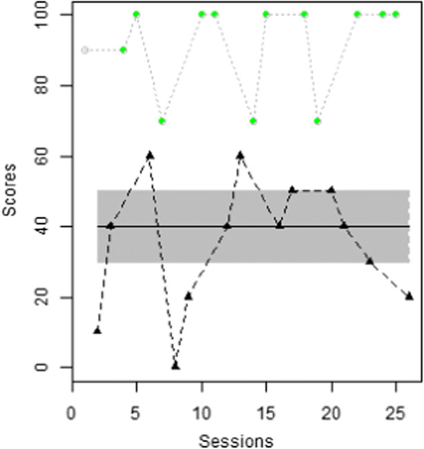
Data for participant Ashley from the Fletcher et al. (2010) study. Theil-Sen trend fitted to Condition A (Number Line), plus a variability band defined by the median absolute deviation. Plots created via https://manolov.shinyapps.io/TrendMAD/, as part of VAIOR (Manolov & Vannest, 2019)

The analyses exemplified in this section demonstrate how to obtain a more thorough and detailed picture of differences between conditions and the consistency of effects, when the effect is clear (participant Ken) and when there is a lot of variability in one condition (Ashley). Further analyses may strengthen the conclusion regarding the difference between the conditions or reveal different characteristics of the data. Additional analyses for this data set can be accessed at https://osf.io/ks4p2.

In Sjolie et al. (2016), a comparison is performed between two versions of speech therapy: with and without exposure to ultrasound visual feedback for postvocalic rhotics (/r/- colored vowels). The authors studied the effects of the two treatments on acquisition, retention, and generalization, hypothesizing that the ultrasound would facilitate acquisition but hinder retention and generalization. Four participants (age 7–9) were studied. Focusing on some of the most interesting and challenging data patterns, Fig. 5 includes the acquisition data for Participant 1003 and the retention data for Participant 1008.

Fig. 5.

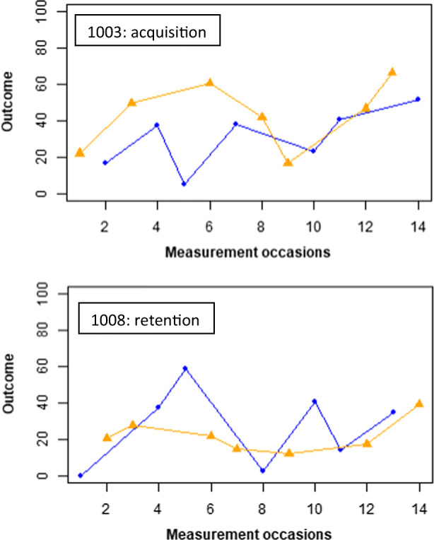
Data gathered by Sjolie et al. (2016) for Participant 1003 during acquisition (upper panel) and Participant 1008 during retention. Condition A (No Ultrasound): Blue. Condition B (Ultrasound): Yellow. Plots created via https://manolov.shinyapps.io/ConsistencyRBD/

Sjolie et al. (2016) report, for acquisition, that

Participant 1003 showed a generally consistent advantage for US sessions over NoUS sessions. Participant 1008 showed signs of acquisition, but no consistent advantage for either US sessions or NoUS sessions. Consistent with the graphical trend, Participant 1003 showed a significant advantage for US sessions over NoUS sessions in acquisition scores (p = .039, d = 0.78); however, the remaining three subjects did not show a significant advantage for either treatment. (p. 69)

In order to provide a more in-depth analysis of the statistically significant result obtained via a randomization test, as reported by the original authors, we compared several different types of quantitative analyses to see if they would yield similar conclusion. For instance, the application of VAIOR (Fig. 6, left panel) indicates that 43% (3 of 7) of the measurements in the condition without ultrasound are outside the variability band constructed around the trend line for this condition. According to the VAIOR criterion for sufficient change, requiring for doubling this percentage (Manolov & Vannest, 2019), at least 86% of the measurements of the condition with ultrasound should be outside the upper limit of the variability band. However, this is the case for only 57% (4 of 7) of the measurements.

Fig. 6.

Data gathered by Sjolie et al. (2016). Left panel: acquisition for Participant 1003; Condition A (No ultrasound): Black triangles. Condition B (Ultrasound): Red, Yellow, and Green Dots. Right panel: retention for Participant 1008; Condition A (Ultrasound): Black triangles. Condition B (No ultrasound): Red, Yellow, and Green Dots. Plots created via https://manolov.shinyapps.io/ATDesign/, as part of VAIOR (Manolov & Vannest, 2019)

A different comparison can be performed, comparing data paths, rather than only actually obtained measurements, using ALIV (Manolov & Onghena, 2018) and the visual structured criterion (Lanovaz et al., 2019). Figure 7 (upper panel) represents this comparison between data paths. With seven measurements per condition, there are 14 measurement occasions and 12 comparisons, which are delimited by the blue vertical lines. Both VSC and ALIV entail omitting the initial value for the ultrasound condition and the last value for the no ultrasound condition. The lines with arrows show a connection between a real data point from one condition to an interpolated point from the other condition. They always originate with the condition denoted as A. Green lines show where condition B (usually the active treatment) is better than condition A (usually the control). If we compare the data paths, it can be seen that the ultrasound condition is superior in 10 of these 12 comparisons. According to the visual structured criterion, one condition being superior to the other in only 10 out of 12 comparisons is not sufficient evidence for superiority, as at least 11 out of 12 is required, following the criteria derived by Lanovaz et al. (2019).

Fig. 7.

Data gathered by Sjolie et al. (2016). Condition A is No ultrasound, whereas Condition B is Ultrasound. Upper panel: acquisition for participant 1003; green marks values greater in Condition B, whereas red marks values greater in Condition A. Upper panel: retention for participant 1008; green marks values greater in Condition A, whereas red marks values greater in Condition B. Plots created via https://manolov.shinyapps.io/ATDesign/, as part of ALIV (Manolov & Onghena, 2018)

When we computed ADISO for the acquisition data from Participant 1003 (Fig. 8, upper panel), we see that the mean difference in favor of the ultrasound condition is 13% correct of all trained items, with the ultrasound condition being superior in 85% of the comparisons. Both these quantifications appear as subtitled in the upper panel of Fig. 8. Finally, to assess the consistency of effects, we can look at the color and the size of the arrows in the upper panel of Fig. 8: there is one red arrow (i.e., superiority of condition A) and the green arrows (i.e., superiority of condition B) are of different lengths. Thus, at least visually, according to Fig. 8, the effect does not seem to be very consistent. In addition, we can also inspect the modified Brinley plot (Fig. 9, left panel). This plot is slightly different from Fig. 3, in that a parallel dashed diagonal line is added, parallel to the solid diagonal line (i.e., no difference) and representing the mean difference between the conditions. The consistency of effect is represented as the vertical distance between the red dots and the dashed diagonal line: the longer the distances, the lower the consistency. Overall, the degree of consistency of effect is quantified as a MAE (equal to 12.75) and as MAE relative to the mean difference (which is the MAPEDIFF quantification). Once again, the effect does not seem to be consistent, considering that the typical distance between the overall mean difference and the difference between conditions within each block is 97% of the overall mean difference (i.e., MAPEDIFF = 0.97). This may be the reason why the statistically significant result from the randomization test, reported by Sjolie et al. (2016), is not detected by VAIOR.

Fig. 8.

Data gathered by Sjolie et al. (2016). Condition A is No ultrasound, whereas Condition B is Ultrasound. Upper panel: acquisition for participant 1003; green marks values greater in Condition B, whereas red marks values greater in Condition A. Upper panel: retention for participant 1008; green marks values greater in Condition A, whereas red marks values greater in Condition B. Plots created via https://manolov.shinyapps.io/ATDesign/ , as part of ADISO (Manolov & Onghena, 2018)

Fig. 9.

Consistency of Effects for the Sjolie et al. (2016) study. The X-axis represents the measurements in condition A (No Ultrasound). The Y-axis represents the measurements in condition B (Ultrasound). Left panel: acquisition for participant 1003. Right panel: retention for participant 1008. The greater the vertical distance between the red dots and the dashed diagonal line, the lower the consistency of differences between conditions across blocks. Plots created via https://manolov.shinyapps.io/Brinley/, as part of the MAPEDIFF quantification (Manolov & Tanious, 2020)

For retention, Sjolie (2016, p. 70) report “a negligible difference between US sessions and NoUS sessions. None of the participants showed a statistically significant advantage for one treatment over the other in retention scores.” It is noteworthy that for Participant 1008 the authors report d = −0.303 and a p-value of .297. Further analyses can reveal whether this lack of statistical significance hides a relevant difference, in favor of the condition without ultrasound. Thus, it should be noted that in the right panel of Fig. 6, representing VAIOR, the condition with ultrasound is treated and depicted as condition A and the condition without ultrasound as condition B. This is opposite to the representation in the left panel of Fig. 6, but we proceeded in this way in order to explore whether there is any evidence for the superiority of the condition without ultrasound. The application of VAIOR reveals that 42% (3 of 7) of the measurements in the condition with ultrasound are outside the variability band constructed around the trend line for this condition. According to the VAIOR criterion (Manolov & Vannest, 2019), at least 84% of the measurements of the condition without ultrasound should be above that variability band. However, just like for acquisition, only 57.14% of the intervention phase data points improve the projected variability band. Using the visual structured criterion (Lanovaz et al., 2019) for comparing data paths, we see that the condition without ultrasound is superior in 8 of the 12 comparisons (as depicted in Fig. 7, bottom panel), which is insufficient evidence. Thus, the conclusion appears to be the same as for acquisition for Participant 1003.

However, when computing ADISO (Fig. 8, lower panel), we see that the mean difference in favor of the no ultrasound condition is 5% correct of all trained items, with the ultrasound condition being superior in only 42% of the comparisons, which is much less that the superiority of the ultrasound condition observed for acquisition for Participant 1003. Finally, the low degree of superiority for retention for Participant 1008 is well-aligned with the results about the consistency of the effect. Focusing on the modified Brinley plot represented on the right panel of Fig. 9, it can be seen that the differences between conditions in each block are relatively far away from the overall mean difference. That is, the vertical distance between the dots and the dashed diagonal line is relatively large, compared to the mean difference. In particular, as indicated in the right panel of Fig. 9, the typical distance between the overall mean difference and the difference between conditions within each block is more than three times (342%) of the overall mean difference.

Overall, the analyses performed here in addition to the ones reported by Sjolie et al. (2016) provide further information about the effectiveness of the two treatments (beyond a quantification expressed as a standardized mean difference) and the consistency of the effect (beyond a p-value). More complete results can be accessed at https://osf.io/ks4p2.

Discussion

We focused on ATDs, a form of SCEDs that have been the focus for several recent data analytical developments. Several of these developments were reviewed and illustrated, with an emphasis on techniques that can be implemented by applied researchers with relatively minimal training in advanced quantitative methods. When using ATDs, several challenges need to be addressed. The specific design and method for generating the alternation sequence for treatment conditions need to be correctly labeled and described with sufficient detail to enable replication. In terms of data analysis, the use of randomization of condition ordering in the design enables the use of an analytical technique allowing for tentative causal inference, but the p-values need to be derived and interpreted correctly. These issues are discussed here.

Need for Transparent Reporting

Labeling the Design

Transparent reporting is necessary with regards to the design used to isolate the effects of the independent variable on the dependent variable that match SCRIBE guidelines for SCEDs (Tate et al., 2016) and CENT guidelines for N-of-1 trials from the health sciences (Vohra et al., 2015). To begin with, the name of the design should be correctly and consistently specified across studies, in order to be able to locate them and include them in systematic reviews and meta-analyses. Difficulties might arise because the same design is sometimes referred to using different names (e.g., as an ATD or a multielement design; Hammond & Gast, 2010; Wolery et al., 2018). Any tentative recommendation that we made in the current manuscript has to consider the tradition for data analysis in different fields. Thus, following Ledford et al. (2019), one option would be to reserve the term “ATD” for designs in which there is an intervention (or two different treatments are being compared), whereas the term “multielement design” could be used when the effect of contextual variables is being studied, such as in functional analysis of problem behavior.

The different variations of ATD (Onghena & Edgington, 1994, 2005) are not equivalent. Thus, it is important to label the type of ATD correctly so applied researchers can analyze the data properly and readers can easily understand (and be able to replicate) the analyses performed. When block randomization of conditions is used, the comparisons to be performed between adjacent conditions are more straightforward because the presence of blocks makes it easier to apply ADISO and it enables using only actually obtained measurements without the need to interpolate as in ALIV. Moreover, the alternation sequences that can possibly be generated using block randomization are not the same as the ones that can arise when using an ATD with restricted randomization. This has implications for the way in which statistical significance is determined (see the later section “Analytical Implications for Randomization Tests”). Further complications in reporting and data analysis arise by the use of combinations of designs (Ledford & Gast, 2018; Moeyaert et al., 2020), such as embedding an ATD within a multiple baseline design or within a reversal design. The main suggestions that we are making here, in relation to ATD in which the effect of a treatment (or more than one treatment) is studied, is to state clearly how the alternation sequence is determined, by specifying whether (1) counterbalancing or randomization is used; and (2) whether blocks are used or there is a restriction imposed on the number of consecutive administrations of the same condition (being explicit about his number). When randomization is used, the terms “ATD with block randomization” and “ATD with restricted randomization” should be used to reduce ambiguity.

Determining the Alternation Sequence

In absence of transparent reporting, it may not be clear exactly what was done to determine the condition sequence (i.e., counterbalancing, randomization, or blocking), and any ambiguity interferes with replication attempts, the reanalysis of the data, and subsequent reviews of the published literature. In relation to randomization, Item 8 of the CENT guidelines require reporting “[w]hether the order of treatment periods was randomised, with rationale, and method used to generate allocation sequence. When applicable, type of randomisation; details of any restrictions (such as pairs, blocking)” (Vohra et al., 2015, p. 4). In the SCRIBE guidelines, Item 8 requires the authors to “[s]tate whether randomization was used, and if so, describe the randomization method and the elements of the study that were randomized” (Tate et al., 2016, p. 140).

It is important not only to state how the alternation sequence was determined, but also to provide additional details. For instance, only stating that counterbalancing was used (e.g., Russell & Reinecke, 2019; Thirumanickam et al., 2018) is often not sufficient to understand and replicate the procedure. Regarding ATDs with block randomization, the most straightforward option is to use this label for the design, or the term “randomized block design” (e.g., Sjolie et al., 2016) and/or to describe the procedure clearly. For example, Lloyd et al. (2018) in particular refer to random assignment between successive pairs of observation, whereas Fletcher et al. (2010) somewhat more ambiguously state that the interventions were administered “semi-randomly” to counterbalance which treatment takes place first each data.

It is possible to further enrich the design by introducing both randomization and counterbalancing. For instance, Maas et al. (2019, p. 3167) state the

[o]rder of conditions within each session was pseudorandomized as follows: The child rolled a die before the first weekly session to determine which condition would be presented first in that session; the following session would have the reverse order. Thus, the order of conditions was counterbalanced by week but randomized across weeks, and each condition was presented an equal number of times in the first and second half of a session (8/16 first, 8/16 second).

Analytical Implications for Randomization Tests

Randomization Scheme for Determining the Alternation Sequence

When randomization is used in the context of any SCED in general and in the context of an ATD in particular, it is important to be clear in describing how the alternation sequence is generated and how the reference distribution for obtaining statistical significance is obtained. It is crucial that the random assignment procedure used for determining the alternation sequence is matched by the randomization performed for obtaining the statistical significance of the result (Edgington, 1980; Levin et al., 2019). For instance, if four days include a morning and an afternoon session, and two conditions take place each day, alternated in random order, this would lead to 2⁴ = 16 possible sequences and it will not be equivalent to dividing eight measurement occasions into two groups of four, which would lead to 8 ! /(4 ! 4!) = 70 possible divisions (Kratochwill & Levin, 1980). The former is a randomized block design, whereas the latter is a completely randomized design (Onghena & Edgington, 2005). An apparent confusion between the two ways of determining the alternation sequence at random, when obtaining a p-value, is present in Hua et al. (2020). Thus, ensuring statistical-conclusion validity (Levin et al., 2019) requires both the presence of randomization when designing and the correspondence between what is done in the design stage and in the analytical stage in which the randomization distribution is constructed (Bulté & Onghena, 2008).

Statistical Inference

Incorporating randomization in the design boosts internal validity and scientific credibility in any type of design, including SCEDs (Edgington, 1975; Kratochwill & Levin, 2010). Moreover, the use of randomization makes possible and valid the use of randomization tests, a kind of statistical test that makes no distributional assumptions and no assumptions about random sampling (Edgington & Onghena, 2007; Levin et al., 2019). The evidence provided by the application of a randomization test to an individual’s data is more closely related to the typical aims in behavioral sciences (Craig & Fisher, 2019). Applied researchers need to be cautious only when performing multiple statistical tests, in relation to potentially committing a Type I error. Finally, statistical inference can be expressed as a confidence interval constructed around an effect size estimate, thanks to inverting the randomization (Michiels et al., 2017).

A potential limitation of randomization tests is that some applied researchers may not be familiar with the correct interpretation of its p-value, but this could also be applicable to other data analytical techniques suggested in the SCED context. For instance, the conservative dual criterion fits a mean line and a trend line to the baseline data and extends them into the intervention phase for comparison (Fisher et al., 2003). The conservative dual criterion can be considered a visual aid, as suggested by its authors, but it actually entails obtaining a p-value (i.e., the probability of observing, only by chance, as many or more intervention points superior to both extended baseline lines, as the number actually observed). In order to avoid repeating the misuses and misinterpretations of p-values (Branch, 2019; Cohen, 1990, 1994; Gigerenzer, 2004; Nickerson, 2000; Wicherts et al., 2016), it is important for applied researchers to know what a null hypothesis is (and is not), when a randomization test is used, and what the statistical inference refers to. In particular, a very small p-value indicates that the difference between the conditions (expressed as difference in means, difference between data paths compared via ALIV, or otherwise, according to the test statistic chosen) is not likely to be obtained only by chance (i.e., if the there is no difference between conditions). The p-value is not a quantification of the reliability or the replicability of the results (Branch, 2014). In fact, p-values do not preclude replications or make them unnecessary, because they are not a tool for extrapolating the results to other participants.

Limitations of the Quantitative Techniques Reviewed and Suggestions for Future Research

It is impossible to recommend a single optimal choice for graphing ATD data or for analyzing these data quantitatively. This is because different graphical representations and analytical techniques provide different types of information: presence or absence of effect, degree of ordinal superiority, average difference between adjacent measurements, average difference between data paths, statistical significance. All these components can be considered together with broader social validity criteria (Horner et al., 2005; Kazdin, 1977) when deciding the degree to which one treatment is superior to another.

Declarations

Conflicts of interest

The authors report no conflicts of interest. Furthermore, the authors have no financial interest for any of the websites mentioned in the manuscript, as they are free to use and the authors do not generate revenue for themselves by the use of the websites.

References

- Barlow DH, Hayes SC. Alternating treatments design: One strategy for comparing the effects of two treatments in a single subject. Journal of Applied Behavior Analysis. 1979;12(2):199–210. doi: 10.1901/jaba.1979.12-199. [DOI] [PMC free article] [PubMed] [Google Scholar]
- Barlow, D. H., Nock, M. K., & Hersen, M. (2009). Single case experimental designs: Strategies for studying behavior change (3rd ed.). Pearson.
- Blampied NM. Analyzing therapeutic change using modified Brinley plots: History, construction, and interpretation. Behavior Therapy. 2017;48(1):115–127. doi: 10.1016/j.beth.2016.09.002. [DOI] [PubMed] [Google Scholar]
- Branch M. Malignant side effects of null-hypothesis significance testing. Theory & Psychology. 2014;24(2):256–277. doi: 10.1177/0959354314525282. [DOI] [Google Scholar]
- Bulté I, Onghena P. An R package for single-case randomization tests. Behavior Research Methods. 2008;40(2):467–478. doi: 10.3758/BRM.40.2.467. [DOI] [PubMed] [Google Scholar]
- Cohen J. Things I have learned (so far) American Psychologist. 1990;45(12):1304–1312. doi: 10.1037/0003-066X.45.12.1304. [DOI] [Google Scholar]
- Cohen J. The Earth is round (p < .05) American Psychologist. 1994;49(12):997–1003. doi: 10.1037/0003-066X.49.12.997. [DOI] [Google Scholar]
- Cox, A., & Friedel, J. E. (2020). Toward an automation of functional analysis interpretation: A proof of concept. Behavior Modification. Advance online publication. 10.1177/0145445520969188 [DOI] [PubMed]
- Craig AR, Fisher WW. Randomization tests as alternative analysis methods for behavior-analytic data. Journal of the Experimental Analysis of Behavior. 2019;111(2):309–328. doi: 10.1002/jeab.500. [DOI] [PMC free article] [PubMed] [Google Scholar]
- Dart EH, Radley KC. The impact of ordinate scaling on the visual analysis of single-case data. Journal of School Psychology. 2017;63:105–118. doi: 10.1016/j.jsp.2017.03.008. [DOI] [PubMed] [Google Scholar]
- De TK, Michiels B, Tanious R, Onghena P. Handling missing data in randomization tests for single-case experiments: A simulation study. Behavior Research Methods. 2020;52(3):1355–1370. doi: 10.3758/s13428-019-01320-3. [DOI] [PubMed] [Google Scholar]
- Dugard, P., File, P., & Todman, J. (2012). Single-case and small-n experimental designs: A practical guide to randomization tests (2nd ed.). Routledge.
- Edgington ES. Statistical inference from N=1 experiments. Journal of Psychology. 1967;65(2):195–199. doi: 10.1080/00223980.1967.10544864. [DOI] [PubMed] [Google Scholar]
- Edgington ES. Randomization tests for one-subject operant experiments. Journal of Psychology. 1975;90(1):57–68. doi: 10.1080/00223980.1975.9923926. [DOI] [Google Scholar]
- Edgington ES. Validity of randomization tests for one-subject experiments. Journal of Educational Statistics. 1980;5(3):235–251. doi: 10.3102/10769986005003235. [DOI] [Google Scholar]
- Edgington ES. Randomized single-subject experimental designs. Behaviour Research & Therapy. 1996;34(7):567–574. doi: 10.1016/0005-7967(96)00012-5. [DOI] [PubMed] [Google Scholar]
- Edgington, E. S., & Onghena, P. (2007). Randomization tests (4th ed.). Chapman & Hall/CRC.
- Fahmie TA, Hanley GP. Progressing toward data intimacy: A review of within-session data analysis. Journal of Applied Behavior Analysis. 2008;41(3):319–331. doi: 10.1901/jaba.2008.41-319. [DOI] [PMC free article] [PubMed] [Google Scholar]
- Falligant JM, Kranak MP, Schmidt JD, Rooker GW. Correspondence between fail-safe k and dual-criteria methods: Analysis of data series stability. Perspectives on Behavior Science. 2020;43(2):303–319. doi: 10.1007/s40614-020-00255-x. [DOI] [PMC free article] [PubMed] [Google Scholar]
- Ferron JM, Joo S-H, Levin JR. A Monte Carlo evaluation of masked visual analysis in response-guided versus fixed-criteria multiple-baseline designs. Journal of Applied Behavior Analysis. 2017;50(4):701–716. doi: 10.1002/jaba.410. [DOI] [PubMed] [Google Scholar]
- Ferron JM, Moeyaert M, Van den Noortgate W, Beretvas SN. Estimating causal effects from multiple-baseline studies: Implications for design and analysis. Psychological Methods. 2014;19(4):493–510. doi: 10.1037/a0037038. [DOI] [PubMed] [Google Scholar]
- Fisher WW, Kelley ME, Lomas JE. Visual aids and structured criteria for improving visual inspection and interpretation of single-case designs. Journal of Applied Behavior Analysis. 2003;36(3):387–406. doi: 10.1901/jaba.2003.36-387. [DOI] [PMC free article] [PubMed] [Google Scholar]
- Fletcher, D., Boon, R. T., & Cihak, D. F. (2010). Effects of the TOUCHMATH program compared to a number line strategy to teach addition facts to middle school students with moderate intellectual disabilities. Education & Training in Autism & Developmental Disabilities, 45(3), 449–458 https://www.jstor.org/stable/23880117. Accessed 3 May 2021.
- Gafurov, B. S., & Levin, J. R. (2020). ExPRT-Excel® package of randomization tests: Statistical analyses of single-case intervention data (Version 4.1, March 2020). Retrieved from https://ex-prt.weebly.com/. Accessed 3 May 2021.
- Gigerenzer G. Mindless statistics. Journal of Socio-Economics. 2004;33(5):587–606. doi: 10.1016/j.socec.2004.09.033. [DOI] [Google Scholar]
- Greenwald AG. Within-subject designs: To use or not to use? Psychological Bulletin. 1976;8(2):314–320. doi: 10.1037/0033-2909.83.2.314. [DOI] [Google Scholar]
- Guyatt GH, Keller JL, Jaeschke R, Rosenbloom D, Adachi JD, Newhouse MT. The n-of-1 randomized controlled trial: Clinical usefulness. Our three-year experience. Annals of Internal Medicine. 1990;112(4):293–299. doi: 10.7326/0003-4819-112-4-293. [DOI] [PubMed] [Google Scholar]
- Hagopian LP, Fisher WW, Thompson RH, Owen-DeSchryver J, Iwata BA, Wacker DP. Toward the development of structured criteria for interpretation of functional analysis data. Journal of Applied Behavior Analysis. 1997;30(2):313–326. doi: 10.1901/jaba.1997.30-313. [DOI] [PMC free article] [PubMed] [Google Scholar]
- Hall SS, Pollard JS, Monlux KD, Baker JM. Interpreting functional analysis outcomes using automated nonparametric statistical analysis. Journal of Applied Behavior Analysis. 2020;53(2):1177–1191. doi: 10.1002/jaba.689. [DOI] [PubMed] [Google Scholar]
- Hammond, D., & Gast, D. L. (2010). Descriptive analysis of single subject research designs: 1983-2007. Education & Training in Autism & Developmental Disabilities, 45(2), 187–202. https://www.jstor.org/stable/23879806. Accessed 3 May 2021.
- Hammond JL, Iwata BA, Rooker GW, Fritz JN, Bloom SE. Effects of fixed versus random condition sequencing during multielement functional analyses. Journal of Applied Behavior Analysis. 2013;46(1):22–30. doi: 10.1002/jaba.7. [DOI] [PubMed] [Google Scholar]
- Hantula DA. Editorial: Replication and reliability in behavior science and behavior analysis: A call for a conversation. Perspectives on Behavior Science. 2019;42(1):1–11. doi: 10.1007/s40614-019-00194-2. [DOI] [PMC free article] [PubMed] [Google Scholar]
- Heyvaert M, Onghena P. Randomization tests for single-case experiments: State of the art, state of the science, and state of the application. Journal of Contextual Behavioral Science. 2014;3(1):51–64. doi: 10.1016/j.jcbs.2013.10.002. [DOI] [Google Scholar]
- Holcombe, A., Wolery, M., & Gast, D. L. (1994). Comparative single subject research: Description of designs and discussion of problems. Topics in Early Childhood and Special Education, 16(1), 168–190. 10.1177/027112149401400111.
- Horner RH, Carr EG, Halle J, McGee G, Odom S, Wolery M. The use of single-subject research to identify evidence-based practice in special education. Exceptional Children. 2005;71(2):165–179. doi: 10.1177/001440290507100203. [DOI] [Google Scholar]
- Horner, R. J., & Odom, S. L. (2014). Constructing single-case research designs: Logic and options. In T. R. Kratochwill & J. R. Levin (Eds.), Single-case intervention research: Methodological and statistical advances (pp. 27–51). American Psychological Association. 10.1037/14376-002.
- Howick, J., Chalmers, I., Glasziou, P., Greenhaigh, T., Heneghan, C., Liberati, A., Moschetti, I., Phillips, B., Thornton, H., Goddard, O., & Hodgkinson, M. (2011). The 2011 Oxford CEBM Levels of Evidence. Oxford Centre for Evidence-Based Medicine. https://www.cebm.ox.ac.uk/resources/levels-of-evidence/ocebm-levels-of-evidence
- Hua Y, Hinzman M, Yuan C, Balint Langel K. Comparing the effects of two reading interventions using a randomized alternating treatment design. Exceptional Children. 2020;86(4):355–373. doi: 10.1177/0014402919881357. [DOI] [Google Scholar]
- Iwata BA, Duncan BA, Zarcone JR, Lerman DC, Shore BA. A sequential, test-control methodology for conducting functional analyses of self-injurious behavior. Behavior Modification. 1994;18(3):289–306. doi: 10.1177/01454455940183003. [DOI] [PubMed] [Google Scholar]
- Jacobs KW. Replicability and randomization test logic in behavior analysis. Journal of the Experimental Analysis of Behavior. 2019;111(2):329–341. doi: 10.1002/jeab.501. [DOI] [PubMed] [Google Scholar]
- Jenson WR, Clark E, Kircher JC, Kristjansson SD. Statistical reform: Evidence-based practice, meta-analyses, and single subject designs. Psychology in the Schools. 2007;44(5):483–493. doi: 10.1002/pits.20240. [DOI] [Google Scholar]
- Johnson AH, Cook BG. Preregistration in single-case design research. Exceptional Children. 2019;86(1):95–112. doi: 10.1177/0014402919868529. [DOI] [Google Scholar]
- Kazdin AE. Assessing the clinical or applied importance of behavior change through social validation. Behavior Modification. 1977;1(4):427–452. doi: 10.1177/014544557714001. [DOI] [Google Scholar]
- Kazdin, A. E. (2011). Single-case research designs: Methods for clinical and applied settings (2nd ed.). Oxford University Press.
- Kennedy, C. H. (2005). Single-case designs for educational research. Pearson.
- Killeen PR. An alternative to null hypothesis statistical tests. Psychological Science. 2005;16(5):345–353. doi: 10.1111/j.0956-7976.2005.01538.x. [DOI] [PMC free article] [PubMed] [Google Scholar]
- Kinney, C. E. L. (2020). A clarification of slope and scale. Behavior Modification. Advance online publication.10.1177/0145445520953366. [DOI] [PubMed]
- Kranak, M. P., Falligant, J. M., & Hausman, N. L. (2021). Application of automated nonparametric statistical analysis in clinical contexts. Journal of Applied Behavior Analysis, 54(2), 824–833. 10.1002/jaba.789. [DOI] [PubMed]
- Kratochwill TR, Hitchcock JH, Horner RH, Levin JR, Odom SL, Rindskopf DM, Shadish WR. Single-case intervention research design standards. Remedial & Special Education. 2013;34(1):26–38. doi: 10.1177/0741932512452794. [DOI] [Google Scholar]
- Kratochwill TR, Levin JR. On the applicability of various data analysis procedures to the simultaneous and alternating treatment designs in behavior therapy research. Behavioral Assessment. 1980;2(4):353–360. [Google Scholar]
- Kratochwill TR, Levin JR. Enhancing the scientific credibility of single-case intervention research: Randomization to the rescue. Psychological Methods. 2010;15(2):124–144. doi: 10.1037/a0017736. [DOI] [PubMed] [Google Scholar]
- Krone T, Boessen R, Bijlsma S, van Stokkum R, Clabbers ND, Pasman WJ. The possibilities of the use of N-of-1 and do-it-yourself trials in nutritional research. PloS One. 2020;15(5):e0232680. doi: 10.1371/journal.pone.0232680. [DOI] [PMC free article] [PubMed] [Google Scholar]
- Lane JD, Gast DL. Visual analysis in single case experimental design studies: Brief review and guidelines. Neuropsychological Rehabilitation. 2014;24(3−4):445–463. doi: 10.1080/09602011.2013.815636. [DOI] [PubMed] [Google Scholar]
- Lane JD, Ledford JR, Gast DL. Single-case experimental design: Current standards and applications in occupational therapy. American Journal of Occupational Therapy. 2017;71(2):7102300010p1–7102300010p9. doi: 10.5014/ajot.2017.022210. [DOI] [PubMed] [Google Scholar]
- Lanovaz M, Cardinal P, Francis M. Using a visual structured criterion for the analysis of alternating-treatment designs. Behavior Modification. 2019;43(1):115–131. doi: 10.1177/0145445517739278. [DOI] [PubMed] [Google Scholar]
- Lanovaz MJ, Huxley SC, Dufour MM. Using the dual-criteria methods to supplement visual inspection: An analysis of nonsimulated data. Journal of Applied Behavior Analysis. 2017;50(3):662–667. doi: 10.1002/jaba.394. [DOI] [PubMed] [Google Scholar]
- Laraway S, Snycerski S, Pradhan S, Huitema BE. An overview of scientific reproducibility: Consideration of relevant issues for behavior science/analysis. Perspectives on Behavior Science. 2019;42(1):33–57. doi: 10.1007/s40614-019-00193-3. [DOI] [PMC free article] [PubMed] [Google Scholar]
- Ledford JR. No randomization? No problem: Experimental control and random assignment in single case research. American Journal of Evaluation. 2018;39(1):71–90. doi: 10.1177/1098214017723110. [DOI] [Google Scholar]
- Ledford JR, Barton EE, Severini KE, Zimmerman KN. A primer on single-case research designs: Contemporary use and analysis. American Journal on Intellectual & Developmental Disabilities. 2019;124(1):35–56. doi: 10.1352/1944-7558-124.1.35. [DOI] [PubMed] [Google Scholar]
- Ledford, J. R., & Gast, D. L. (2018). Combination and other designs. In D. L. Gast & J. R. Ledford (Eds.), Single case research methodology: Applications in special education and behavioral sciences (3rd ed., pp. 335–364). Routledge.
- Levin JR, Ferron JM, Gafurov BS. Additional comparisons of randomization-test procedures for single-case multiple-baseline designs: Alternative effect types. Journal of School Psychology. 2017;63:13–34. doi: 10.1016/j.jsp.2017.02.003. [DOI] [PubMed] [Google Scholar]
- Levin, J. R., Ferron, J. M., & Gafurov, B. S. (2020). Investigation of single-case multiple-baseline randomization tests of trend and variability. Educational Psychology Review. Advance online publication. 10.1007/s10648-020-09549-7
- Levin JR, Ferron JM, Kratochwill TR. Nonparametric statistical tests for single-case systematic and randomized ABAB…AB and alternating treatment intervention designs: New developments, new directions. Journal of School Psychology. 2012;50(5):599–624. doi: 10.1016/j.jsp.2012.05.001. [DOI] [PubMed] [Google Scholar]
- Levin JR, Kratochwill TR, Ferron JM. Randomization procedures in single-case intervention research contexts: (Some of) “the rest of the story”. Journal of the Experimental Analysis of Behavior. 2019;112(3):334–348. doi: 10.1002/jeab.558. [DOI] [PubMed] [Google Scholar]
- Lloyd BP, Finley CI, Weaver ES. Experimental analysis of stereotypy with applications of nonparametric statistical tests for alternating treatments designs. Developmental Neurorehabilitation. 2018;21(4):212–222. doi: 10.3109/17518423.2015.1091043. [DOI] [PubMed] [Google Scholar]
- Maas E, Gildersleeve-Neumann C, Jakielski K, Kovacs N, Stoeckel R, Vradelis H, Welsh M. Bang for your buck: A single-case experimental design study of practice amount and distribution in treatment for childhood apraxia of speech. Journal of Speech, Language, & Hearing Research. 2019;62(9):3160–3182. doi: 10.1044/2019_JSLHR-S-18-0212. [DOI] [PubMed] [Google Scholar]
- Maggin DM, Cook BG, Cook L. Using single-case research designs to examine the effects of interventions in special education. Learning Disabilities Research & Practice. 2018;33(4):182–191. doi: 10.1111/ldrp.12184. [DOI] [Google Scholar]
- Manolov R. A simulation study on two analytical techniques for alternating treatments designs. Behavior Modification. 2019;43(4):544–563. doi: 10.1177/0145445518777875. [DOI] [PubMed] [Google Scholar]
- Manolov R, Onghena P. Analyzing data from single-case alternating treatments designs. Psychological Methods. 2018;23(3):480–504. doi: 10.1037/met0000133. [DOI] [PubMed] [Google Scholar]
- Manolov, R., & Tanious, R. (2020). Assessing consistency in single-case data features using modified Brinley plots. Behavior Modification. Advance online publication. 10.1177/0145445520982969 [DOI] [PubMed]
- Manolov, R., Tanious, R., De, T. K., & Onghena, P. (2020). Assessing consistency in single-case alternation designs. Behavior Modification. Advance online publication. 10.1177/0145445520923990 [DOI] [PubMed]
- Manolov, R., & Vannest, K. (2019). A visual aid and objective rule encompassing the data features of visual analysis. Behavior Modification. Advance online publication. 10.1177/0145445519854323 [DOI] [PubMed]
- Michiels B, Heyvaert M, Meulders A, Onghena P. Confidence intervals for single-case effect size measures based on randomization test inversion. Behavior Research Methods. 2017;49(1):363–381. doi: 10.3758/s13428-016-0714-4. [DOI] [PubMed] [Google Scholar]
- Michiels B, Onghena P. Randomized single-case AB phase designs: Prospects and pitfalls. Behavior Research Methods. 2019;51(6):2454–2476. doi: 10.3758/s13428-018-1084-x. [DOI] [PubMed] [Google Scholar]
- Moeyaert M, Akhmedjanova D, Ferron J, Beretvas SN, Van den Noortgate W. Effect size estimation for combined single-case experimental designs. Evidence-Based Communication Assessment & Intervention. 2020;14(1−2):28–51. doi: 10.1080/17489539.2020.1747146. [DOI] [Google Scholar]
- Moeyaert M, Ugille M, Ferron J, Beretvas SN, Van den Noortgate W. The influence of the design matrix on treatment effect estimates in the quantitative analyses of single-case experimental designs research. Behavior Modification. 2014;38(5):665–704. doi: 10.1177/0145445514535243. [DOI] [PubMed] [Google Scholar]
- Nickerson RS. Null hypothesis significance testing: A review of an old and continuing controversy. Psychological Methods. 2000;5(2):241–301. doi: 10.1037/1082-989X.5.2.241. [DOI] [PubMed] [Google Scholar]
- Nikles, J., & Mitchell, G. (Eds.). (2015). The essential guide to N-of-1 trials in health. Springer.
- Ninci, J. (2019). Single-case data analysis: A practitioner guide for accurate and reliable decisions. Behavior Modification. Advance online publication. 10.1177/0145445519867054 [DOI] [PubMed]
- Ninci J, Vannest KJ, Willson V, Zhang N. Interrater agreement between visual analysts of single-case data: A meta-analysis. Behavior Modification. 2015;39(4):510–541. doi: 10.1177/0145445515581327. [DOI] [PubMed] [Google Scholar]
- Onghena, P. (2020). One by one: The design and analysis of replicated randomized single-case experiments. In R. van de Schoot & M. Miočević (Eds.), Small sample size solutions: A guide for applied researchers and practitioners (pp. 87–101). Routledge.
- Onghena P, Edgington ES. Randomization tests for restricted alternating treatments designs. Behaviour Research & Therapy. 1994;32(7):783–786. doi: 10.1016/0005-7967(94)90036-1. [DOI] [PubMed] [Google Scholar]
- Onghena P, Edgington ES. Customization of pain treatments: Single-case design and analysis. Clinical Journal of Pain. 2005;21(1):56–68. doi: 10.1097/00002508-200501000-00007. [DOI] [PubMed] [Google Scholar]
- Onghena P, Michiels B, Jamshidi L, Moeyaert M, Van den Noortgate W. One by one: Accumulating evidence by using meta-analytical procedures for single-case experiments. Brain Impairment. 2018;19(1):33–58. doi: 10.1017/BrImp.2017.25. [DOI] [Google Scholar]
- Perone M. Statistical inference in behavior analysis: Experimental control is better. The Behavior Analyst. 1999;22(2):109–116. doi: 10.1007/BF03391988. [DOI] [PMC free article] [PubMed] [Google Scholar]
- Petursdottir AI, Carr JE. Applying the taxonomy of validity threats from mainstream research design to single-case experiments in applied behavior analysis. Behavior Analysis in Practice. 2018;11(3):228–240. doi: 10.1007/s40617-018-00294-6. [DOI] [PMC free article] [PubMed] [Google Scholar]
- Pustejovsky, J. E., Swan, D. M., & English, K. W. (2019). An examination of measurement procedures and characteristics of baseline outcome data in single-case research. Behavior Modification. Advance online publication. 10.1177/0145445519864264 [DOI] [PubMed]
- Radley KC, Dart EH, Wright SJ. The effect of data points per x- to y-axis ratio on visual analysts evaluation of single-case graphs. School Psychology Quarterly. 2018;33(2):314–322. doi: 10.1037/spq0000243. [DOI] [PubMed] [Google Scholar]
- Riley-Tillman, T. C., Burns, M. K., & Kilgus, S. P. (2020). Evaluating educational interventions: Single-case design for measuring response to intervention (2nd ed.). Guilford Press.
- Russell SM, Reinecke D. Mand acquisition across different teaching methodologies. Behavioral Interventions. 2019;34(1):127–135. doi: 10.1002/bin.1643. [DOI] [Google Scholar]
- Shadish WR, Hedges LV, Pustejovsky JE. Analysis and meta-analysis of single-case designs with a standardized mean difference statistic: A primer and applications. Journal of School Psychology. 2014;52(2):123–147. doi: 10.1016/j.jsp.2013.11.005. [DOI] [PubMed] [Google Scholar]
- Shadish WR, Kyse EN, Rindskopf DM. Analyzing data from single-case designs using multilevel models: New applications and some agenda items for future research. Psychological Methods. 2013;18(3):385–405. doi: 10.1037/a0032964. [DOI] [PubMed] [Google Scholar]
- Shadish WR, Sullivan KJ. Characteristics of single-case designs used to assess intervention effects in 2008. Behavior Research Methods. 2011;43(4):971–980. doi: 10.3758/s13428-011-0111-y. [DOI] [PubMed] [Google Scholar]
- Sidman, M. (1960). Tactics of scientific research. Basic Books.
- Simmons JP, Nelson LD, Simonsohn U. False-positive psychology: Undisclosed flexibility in data collection and analysis allows presenting anything as significant. Psychological Science. 2011;22(11):1359–1366. doi: 10.1177/0956797611417632. [DOI] [PubMed] [Google Scholar]
- Sjolie GM, Leveque MC, Preston JL. Acquisition, retention, and generalization of rhotics with and without ultrasound visual feedback. Journal of Communication Disorders. 2016;64:62–77. doi: 10.1016/j.jcomdis.2016.10.003. [DOI] [PMC free article] [PubMed] [Google Scholar]
- Smith JD. Single-case experimental designs: A systematic review of published research and current standards. Psychological Methods. 2012;17(4):510–550. doi: 10.1037/a0029312. [DOI] [PMC free article] [PubMed] [Google Scholar]
- Solmi F, Onghena P, Salmaso L, Bulté I. A permutation solution to test for treatment effects in alternation design single-case experiments. Communications in Statistics—Simulation & Computation. 2014;43(5):1094–1111. doi: 10.1080/03610918.2012.725295. [DOI] [Google Scholar]
- Solomon BG. Violations of assumptions in school-based single-case data: Implications for the selection and interpretation of effect sizes. Behavior Modification. 2014;38(4):477–496. doi: 10.1177/0145445513510931. [DOI] [PubMed] [Google Scholar]
- Tanious, R., & Onghena, P. (2020). A systematic review of applied single-case research published between 2016 and 2018: Study designs, randomization, data aspects, and data analysis. Behavior Research Methods. Advance online publication. 10.3758/s13428-020-01502-4 [DOI] [PubMed]
- Tate RL, Perdices M, Rosenkoetter U, Shadish W, Vohra S, Barlow DH, Horner R, Kazdin A, Kratochwill TR, McDonald S, Sampson M, Shamseer L, Togher L, Albin R, Backman C, Douglas J, Evans JJ, Gast D, Manolov R, Mitchell G, et al. The Single-Case Reporting guideline In BEhavioural interventions (SCRIBE) 2016 statement. Journal of School Psychology. 2016;56:133–142. doi: 10.1016/j.jsp.2016.04.001. [DOI] [PubMed] [Google Scholar]
- Tate RL, Perdices M, Rosenkoetter U, Wakim D, Godbee K, Togher L, McDonald S. Revision of a method quality rating scale for single-case experimental designs and n-of-1 trials: The 15-item Risk of Bias in N-of-1 Trials (RoBiNT) Scale. Neuropsychological Rehabilitation. 2013;23(5):619–638. doi: 10.1080/09602011.2013.824383. [DOI] [PubMed] [Google Scholar]
- Thirumanickam A, Raghavendra P, McMillan JM, van Steenbrugge W. Effectiveness of video-based modelling to facilitate conversational turn taking of adolescents with autism spectrum disorder who use AAC. AAC: Augmentative & Alternative Communication. 2018;34(4):311–322. doi: 10.1080/07434618.2018.1523948. [DOI] [PubMed] [Google Scholar]
- Van den Noortgate W, Onghena P. Hierarchical linear models for the quantitative integration of effect sizes in single-case research. Behavior Research Methods, Instruments, & Computers. 2003;35(1):1–10. doi: 10.3758/BF03195492. [DOI] [PubMed] [Google Scholar]
- Vannest KJ, Parker RI, Davis JL, Soares DA, Smith SL. The Theil–Sen slope for high-stakes decisions from progress monitoring. Behavioral Disorders. 2012;37(4):271–280. doi: 10.1177/019874291203700406. [DOI] [Google Scholar]
- Vohra S, Shamseer L, Sampson M, Bukutu C, Schmid CH, Tate R, Nikles J, Zucker DR, Kravitz R, Guyatt G, Altman DG, Moher D. CONSORT extension for reporting N-of-1 trials (CENT) 2015 Statement. British Medical Journal. 2015;350:h1738. doi: 10.1136/bmj.h1738. [DOI] [PubMed] [Google Scholar]
- Weaver ES, Lloyd BP. Randomization tests for single case designs with rapidly alternating conditions: An analysis of p-values from published experiments. Perspectives on Behavior Science. 2019;42(3):617–645. doi: 10.1007/s40614-018-0165-6. [DOI] [PMC free article] [PubMed] [Google Scholar]
- What Works Clearinghouse. (2020). What works clearinghouse standards handbook, version 4.1. U.S. Department of Education, Institute of Education Sciences, National Center for Education Evaluation & Regional Assistance. https://ies.ed.gov/ncee/wwc/handbooks. Accessed 3 May 2021.
- Wicherts JM, Veldkamp CL, Augusteijn HE, Bakker M, van Aert RC, Van Assen MA. Degrees of freedom in planning, running, analyzing, and reporting psychological studies: A checklist to avoid p-hacking. Frontiers in Psychology. 2016;7:1–12. doi: 10.3389/fpsyg.2016.01832. [DOI] [PMC free article] [PubMed] [Google Scholar]
- Wilkinson L, The Task Force on Statistical Inference Statistical methods in psychology journals: Guidelines and explanations. American Psychologist. 1999;54(8):694–704. doi: 10.1037/0003-066X.54.8.594. [DOI] [Google Scholar]
- Wolery M, Busick M, Reichow B, Barton EE. Comparison of overlap methods for quantitatively synthesizing single-subject data. Journal of Special Education. 2010;44(1):18–29. doi: 10.1177/0022466908328009. [DOI] [Google Scholar]
- Wolery, M., Gast, D. L., & Ledford, J. R. (2018). Comparative designs. In D. L. Gast & J. R. Ledford (Eds.), Single case research methodology: Applications in special education and behavioral sciences (3rd ed., pp. 283–334). Routledge.
- Wolfe, K., & McCammon, M. N. (2020). The analysis of single-case research data: Current instructional practices. Journal of Behavioral Education. Advance online publication. 10.1007/s10864-020-09403-4
- Wolfe K, Seaman MA, Drasgow E, Sherlock P. An evaluation of the agreement between the conservative dual-criterion method and expert visual analysis. Journal of Applied Behavior Analysis. 2018;51(2):345–351. doi: 10.1002/jaba.453. [DOI] [PubMed] [Google Scholar]
- Zucker DR, Ruthazer R, Schmid CH. Individual (N-of-1) trials can be combined to give population comparative treatment effect estimates: Methodologic considerations. Journal of Clinical Epidemiology. 2010;63(12):1312–1323. doi: 10.1016/j.jclinepi.2010.04.020. [DOI] [PMC free article] [PubMed] [Google Scholar]
Associated Data
This section collects any data citations, data availability statements, or supplementary materials included in this article.
Data Availability Statement
The data used for the illustrations are available from https://osf.io/ks4p2/