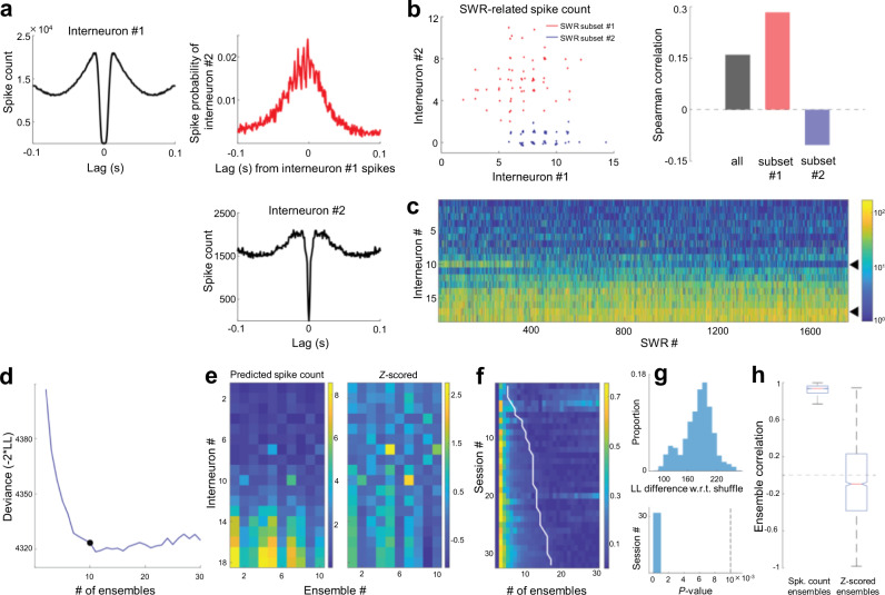
Fig. 9. Heterogeneity in SWR-related interneuronal activity.
a Auto- and cross-correlograms of two example interneurons computed from spikes emitted during SWRs. Note the highly rhythmic spike relationship throughout SWRs. b Left: Spike counts of example interneurons (shown in a)) in two subsets of SWRs (red, blue) recorded in the same session. Each dot indicates a single SWR. Right: SWR-related spike count correlations in all SWRs (black) and the two subsets (red, blue) highlighted on the left. c SWR-related spike counts of all interneurons recorded in an example session, sorted according to mean firing rate. Black triangles highlight interneurons shown in (a) and (b). d The spike count matrix in (c) was modeled using a generalized mixture model with Poisson observations (“ensembles”). The optimal number of ensembles was identified as the point of maximum curvature in the cross-validated deviance curve (−2 × log-likelihood). e Left: Model-predicted interneuron spike counts in each ensemble. Right: Spike counts are expressed as Z-scores with reference to spike count distributions across all SWRs. f Deviance curves (rows, normalized between 0 and 1) in all sessions used for the analysis in Fig. 7g. The white line denotes the optimal number of interneuron ensembles. g Top: For each selected model, log-likelihood on the test set was compared against a surrogate dataset in which spike counts were shuffled across SWRs for each individual interneuron (see “Methods”), thereby yielding a P-value (bottom; n = 32 sessions, two-sided, one-sample t-test). Dashed vertical line indicates P = 0.01. h Ensemble-ensemble correlations (n = 2197 pairs) when the contributions of interneurons were expressed as predicted spike counts (left) or Z-scored (right). The central mark and edges indicate the median and the 25th/75th percentiles, respectively, while the whiskers extend to the most extreme data points.

