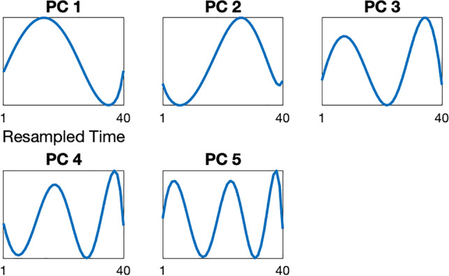
Fig. 2.

The top five principal component eigenvectors (PCs), representing basis functions that explain the majority of variance in the submovement velocity versus time curve (i.e., submovement shape). Submovements (see Fig. 1 for examples) can be partially reconstructed by a linear combination of the five principal component vectors shown. Each panel provides a visualization of an eigenvector, with the element values displayed on the y-axis for each dimension of the 40-dimensional vector. PCs 1 and 2 demonstrate a single sine wave cycle with a peak in the first half and second half of the submovement, respectively. PCs 3, 4, and 5 have increasing cycles in half-cycle increments, with 1.5, 2, and 2.5 cycles, respectively