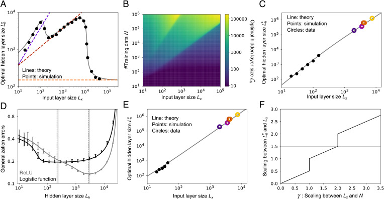
Fig. 4.

Model behavior under maximum-likelihood estimation. (A) Relationship between the input-layer size, L_x, and the optimal hidden-layer size, $L_h^{*}$, at a fixed sample size ($N=30,000$). Gray lines are found by optimizing Eq. 12 with respect to L_h; dashed lines are the asymptotic expression derived in SI Appendix, section 5.1. (B) Optimal hidden-layer size, $L_h^{*}$, as a function of the input-layer size, L_x, and the sample size, N, from Eq. 12. (C) Scaling at $N=1.65L_x^{1.96}$ . Gray line is theory; black points are from simulations; colored circles are the experimental data from Fig. 1A. Simulations were done only for low L_x, due to the computational cost of the simulations when L_x is large. (D) Relationship between the hidden-layer size, L_h, and the generalization error, ϵ_gen, under the logistic activation function (black), and ReLU (gray), at L_x = 50 and $N=30,000$. Lines are theory; bars are from simulations. Vertical lines mark the minima (solid, theory; dashed, simulations). Error bars are the SD over 10 simulations. (E) Scaling for the logistic activation function with $N=240L_x^{1.96}$. Gray line is theory; black points are from simulations; colored circles are the experimental data from Fig. 1A. As in C, simulations were done only for low L_x, due to the computational cost of the simulations when L_x is large. (F) Analytical estimation of the $L_h^{*}$ - L_x scaling versus the L_x-N scaling (y axis, coefficient β in the scaling $L_x^{*}\propto L_x^{\beta }$; x axis, coefficient γ in the scaling $L_x\propto N^{\gamma }$; see SI Appendix, section 5.1 for details). The gray horizontal line is the 3/2 scaling from Fig. 1A. As in Fig. 3, the teacher network had a hidden-layer size of 500, with a ReLU nonlinearity, and the noise was set to ${\sigma }_t^2=0.1$.