The entorhinal cortex of the monkey: VI. Organization of projections from the hippocampus, subiculum, presubiculum, and parasubiculum

Abstract

The organization of projections from the macaque monkey hippocampus, subiculum, presubiculum, and parasubiculum to the entorhinal cortex was analyzed using anterograde and retrograde tracing techniques. Projections exclusively originate in the CA1 field of the hippocampus and in the subiculum, presubiculum, and parasubiculum. The CA1 and subicular projections terminate most densely in Layers V and VI of the entorhinal cortex, with sparser innervation of the deep portion of Layers III and II. Entorhinal projections from CA1 and the subiculum are topographically organized such that a rostrocaudal axis of origin is related to a medial-to-lateral axis of termination. A proximodistal axis of origin in CA1 and distoproximal axis in subiculum are related to a rostrocaudal axis of termination in the entorhinal cortex. The presubiculum sends a dense, bilateral projection to caudal parts of the entorhinal cortex. This projection terminates most densely in Layer III with sparser termination in Layers I, II, and V. The same parts of entorhinal cortex receive a dense projection from the parasubiculum. This projection terminates in Layers III and II. Both presubicular and parasubicular projections demonstrate the same longitudinal topographic organization as the projections from CA1 and the subiculum. These studies demonstrate that: (a) hippocampal and subicular inputs to the entorhinal cortex in the monkey are organized similar to those described in nonprimate species; (b) the topographic organization of the projections from the hippocampus and subicular areas matches that of the reciprocal projections from the entorhinal cortex to the hippocampus and the subicular areas.

1 |. INTRODUCTION

The hippocampal formation plays an essential role in normal memory function (Mishkin, 1978; Squire, 1986). As part of ongoing studies designed to investigate the functional anatomy of the monkey hippocampal formation, we have evaluated the development, cytoarchitectonic organization, extrinsic and intrinsic connectivity, and intrahippocampal circuitry of the entorhinal cortex (Amaral, Insausti, & Cowan, 1987; Amaral, Kondo, & Lavenex, 2014; Chrobak & Amaral, 2007; Insausti, Amaral, & Cowan, 1987a; Kondo, Lavenex, & Amaral, 2008, 2009; Witter & Amaral, 1991;Witter, Van Hoesen, & Amaral, 1989). In the macaque monkey, the entorhinal cortex (Amaral et al., 1987) receives direct projections from several polysensory areas of the neocortex (Insausti et al., 1987a), as well as from subcortical domains such at the amygdaloid complex (Pitkanen, Kelly, & Amaral, 2002). The entorhinal cortex thus provides the major route through which sensory information, that is presumably involved in the development of long-term memory, reaches the hippocampal formation (Nilssen, Doan, Nigro, Ohara, & Witter, 2019). This information is conveyed to the dentate gyrus, hippocampus and subiculum via the so-called perforant path projections (Witter & Amaral, 1991).

In previous studies (Witter & Amaral, 1991; Witter, Van Hoesen, & Amaral, 1989), we examined the laminar and topographic organization of the monkey entorhinal perforant path projections to hippocampal structures. We confirmed in the monkey, the original description by Steward and Scoville (1976) in the rat, that Layer II cells (and to a lesser extent Layer VI cells) of the entorhinal cortex project to the dentate gyrus and to the CA3/CA2 fields of the hippocampus whereas Layer III cells, and to a lesser extent Layer V cells, project to CA1 and to the subiculum. We further demonstrated that the perforant path projections are organized in a highly distinctive topographic fashion. The topography had both rostrocaudal and mediolateral components, again similar to what has been detailed in rodents (van Groen, Kadish, & Wyss, 2002; Witter, Chan-Palay, & Köhler, 1989). The lateral portion of the entorhinal cortex (the portion lying adjacent to the rhinal sulcus along the full rostrocaudal extent of the entorhinal cortex) projects to caudal levels of the dentate gyrus, hippocampus, and the subiculum. Progressively more medial portions of the entorhinal cortex project to more rostral levels of these fields. Within the rostrocaudally oriented bands of Layer II cells projecting to a particular level of the dentate gyrus and CA3/CA2, the cells located rostrally (in ER for example), originate a projection that terminates superficially in the molecular layer of the dentate gyrus and the stratum lacunosum-moleculare of CA3/CA2. Projections from Layer II cells located caudally terminate deeper in these layers. The Layer III cells that project to CA1 and the subiculum also terminate differentially depending on their rostrocaudal location. In this case, however, terminal fields are not organized in a laminar fashion but are distributed to different transverse portions of CA1 and the subiculum. Layer III cells located rostrally in the entorhinal cortex project to the CA1/subiculum border zone whereas cells located more caudally in the entorhinal cortex project to the portion of CA1 that is closer to CA2 and to that part of the subiculum that is closer to the presubiculum.

Overall, these topographical gradients do not adhere to the seven distinct cytoarchitectonic divisions in the macaque monkey (Amaral et al., 1987), but rather indicate an overall gradient along a rostrolateral to caudomedial axis. The goal of the present study was to investigate the organization of hippocampal projections back to the entorhinal cortex. In particular, we aimed to determine whether the hippocampal projections to the entorhinal cortex respected the topography established by the perforant path. If so, one would predict that caudal levels of the hippocampal formation would project to the most lateral portion of the entorhinal cortex and that different transverse portions of the same rostrocaudal level of CA1 and the subiculum would project to different rostrocaudal levels of the entorhinal cortex.

Several studies carried out in nonprimates indicate that the hippocampus, the subiculum the presubiculum and the parasubiculum do indeed contribute substantial projections to the entorhinal cortex. Early on, Shipley (1974, 1975) used silver degeneration methods to demonstrate that the presubiculum originates a topographically organized projection to the medial entorhinal cortex of the guinea pig. Köhler, Shipley, Srebro, and Harkmark (1978) confirmed this finding in the mouse and rat using the retrograde tracer, horseradish peroxidase. Swanson and Cowan (1977) used the autoradiographic method with small injections of ³H-amino acids into each of the fields of the hippocampal formation and reported that the entorhinal cortex received projections from the CA3, CA2, and CA1 fields of the hippocampus and from the presubiculum and parasubiculum. A later study corroborated projections from CA1 to the entorhinal cortex (Cenquizca & Swanson, 2007) and more recently two studies described a direct projection from CA2 to the entorhinal cortex in rodents (Rowland et al., 2013) and cat (Ino, Kaneko, & Mizuno, 2001). Subicular projections to the entorhinal cortex have been reported in the guinea pig (Sorensen & Shipley, 1979), rodents (Cembrowski et al., 2018; Honda, Umitsu, & Ishizuka, 1999; Kloosterman, Witter, & Van Haeften, 2003; Köhler, 1985), rabbit (Honda & Shibata, 2017), and cat (Ino et al., 2001; van Groen & Wyss, 1990a). Entorhinal inputs from the rat presubiculum and parasubiculum have been described in detail using the anterograde tracers Phaseolus vulgaris Leucoagglutinin (PHA-L) and biotinylated dextran-amine in rat (Caballero-Bleda & Witter, 1993, 1994; Honda & Ishizuka, 2004; Köhler, 1985; van Haeften, Wouterlood, Jorritsma-Byham, & Witter, 1997), rabbit (Honda & Shibata, 2017), and cat (Ino et al., 2001).

In the monkey, it has been reported (Rosene and Van Hoesen 1977; Saunders and Rosene 1988) that CA1, the subiculum, and the presubiculum project to the entorhinal cortex. The topography of these projections, however, was not established. The major goals of the work reported here was to reinvestigate the hippocampal, subicular, and pre- and parasubicular projections to all regions of the entorhinal cortex and to determine their laminar and topographic organization.

2 |. MATERIALS AND METHODS

The results presented in this article are based on the analysis of experiments with injections of a variety of anterograde and retrograde tracers into the hippocampal formation of 41 mature Macaca fascicularis monkeys of both sexes weighing approximately 3.5 kg at the time of surgery (Table 1). All experimental procedures were approved by the Institutional Animal Care and Use Committee at UC Davis. The material used for the present manuscript was taken from an extensive series of experimental cases prepared in the laboratory of DGA over a long period of time. However, all data analysis was done in the period 1996/97 and all fluorescent plots were made either directly after processing of the relevant brains or using series of sections stored at −20 that were only thawed and plotted once in the period 1996/97. The original manuscript was submitted in 1998; for the current resubmission we prepared a few additional figures of retrograde fluorescent cases based on the original plotted data (Figures 4 and 5) and took digital brightfield images of some nonfluorescent injection sites of anterogradely transported tracers (Figure 10).

TABLE 1.

Summary of anterograde and retrograde tracer injections

Anterograde tracers
Experiment	Location	Tracer	Volume	Survival period
DM-1	PaS	3H-AA	100 nl Prol./Leuc.	7 days
DM-2	PaS	3H-AA	100 nl Prol./Leuc.	7 days
DM-17	PaS	3H-AA	100 nl Prol./Leuc.	7 days
DM-9	PrS	3H-AA	100 nl Prol./Leuc.	7 days
DM-41	PrS	3H-AA	100 nl Prol./Leuc.	7 days
MF-7	PrS	3H-AA	50 nl Prol./Leuc.	7 days
MF-9	PrS	3H-AA	50 nl Prol./Leuc.	7 days
DM-35	PrS	3H-AA	100 nl Prol./Leuc.	14 days
DM-16	PrS	3H-AA	3× 200 nl Prol./Leuc.	7 days
FCP-3	CA1/Sub	3H-AA	1 μl Prol./Leuc.	14 days
MF-17	CA1/Sub	3H-AA	50 nl Prol./Leuc.	7 days
DM-30	Sub	3H-AA	100 nl Prol./Leuc.	14 days
MF-19	Sub	3H-AA	50 nl Prol./Leuc.	7 days
DM-7	Sub	3H-AA	60 nl Prol./Leuc.	7 days
MF-1	CA1	3H-AA	50 nl Prol./Leuc.	7 days
M-5–84	CA1	3H-AA	100 nl Prol./Leuc.	14 days
DM-33	CA1	3H-AA	100 nl Prol./Leuc.	14 days
M-5–89	CA1	PHA-L	5 μamps 45 min	14 days
M-21–91	CA1	PHA-L	5 μamps 45 min	14 days
M-30–92	CA1	PHA-L	5 μamps 45 min	14 days
MF-18	CA3	3H-AA	50 nl Prol./Leuc.	7 days
MF-13	CA3	3H-AA	50 nl Prol./Leuc.	7 days
MF-3	CA3	3H-AA	50 nl Prol./Leuc.	7 days
DM-4	CA3	3H-AA	60 nl Prol./Leuc.	7 days
M-1–92	CA3	PHA-L	5 μamps 45 min	14 days
M-2–92	CA3	PHA-L	5 μamps 45 min	14 days
M-2–91	CA3	PHA-L	5 μamps 45 min	14 days
Retrograde tracers
Experiment	Location	Tracer	Volume	Survival period
IM-1	EC	1% WGA-HRP	300 nl	2 days
IM-3	EC	1% WGA-HRP	200 nl	2 days
IM-4	EC	1% WGA-HRP	100 nl	2 days
IM-6	EC	1% WGA-HRP	100 nl	2 days
IM-7	EC	1% WGA-HRP	100 nl	2 days
IM-8	EC	1% WGA-HRP	100 nl	2 days
IM-10	EC	1% WGA-HRP	100 nl	2 days
DM-45	EC	1% WGA-HRP	100 nl	2 days
M-4–86	EC	1% WGA-HRP	100 nl	3 days
M-11–90	EC	3% DY	500 nl	14 days
M-11–90	EC	2% FB	500 nl	14 days
M-1–90	EC	2% FB	500 nl	14 days
M-8–90	EC	3% DY	500 nl	14 days
M-9–90	EC	3% DY	500 nl	14 days

FIGURE 4.

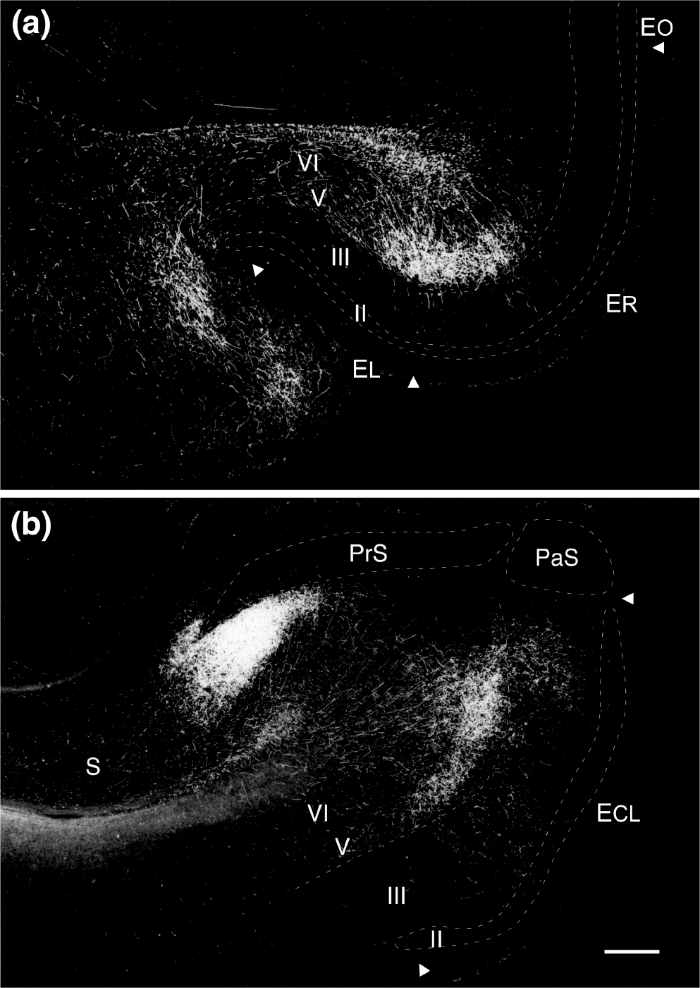
The distribution of retrogradely labeled neurons in two cases with injections in medial parts of EC. a–d, four coronal sections, taken from different levels along the rostrocaudal axis from an injection in rostromedial parts of EI (IM-4). e–h, four coronal sections, taken from different levels along the rostrocaudal axis from an injection caudomedially in EI (M-4–86). Note the presence of labeled neurons in CA1 and subiculum, only in rostral levels (a,b and e,f respectively; see also Figure 6 for the full representation along the rostrocaudal axis). Labeled neurons in case IM-4 are mainly present distally in CA1and in the adjacent proximal subiculum (a–c), whereas in case of the more caudal injection (M-4–86), labeled neurons are mainly present in proximal CA1 and distal subiculum (e,f). Note the presence of labeling in the pre- and parasubiculum only in case M-4–86 (e,f) [Color figure can be viewed at wileyonlinelibrary.com]

FIGURE 5.

The distribution of retrogradely labeled neurons in two cases with injections in lateral parts of EC. a–d, four coronal sections, taken from different levels along the rostrocaudal axis from an injection rostrolaterally involving the border region between ER and EI (M11–90 DY). e–h, four coronal sections, taken from different levels along the rostrocaudal axis from an injection caudolaterally in EC, with some perirhinal involvement (M-8–90). Note the presence of labeled neurons in CA1 and subiculum along the longitudinal extents but also compare with the full lengths presented in the unfolded maps in Figure 6. The latter figure shows that the most lateral of the two injections (M-8–90) does result in retrogradely labeled neurons at even more caudal levels than shown in Panel h. Labeled neurons in case M-11–90 DY are mainly present distally in CA1and in the adjacent proximal subiculum (c,d), whereas in the case of the more caudal injection (M-8–90), labeled neurons are also present in proximal CA1 and distal subiculum (e,f). Note the presence of labeling in pre- and parasubiculum only in case M-8–90 (g,h) [Color figure can be viewed at wileyonlinelibrary.com]

FIGURE 10.

Coronal sections of the hippocampal formation showing three representative anterograde injection sites. (a) PHA-L injection in proximal CA1 (case M-5–89; see also Figure 9). (b) PHA-L injection (Gallyas counterstained) in distal CA1 (M-30–92; see also Figure 9). (c) Tritiated amino acid injection (Nissl counterstained) in the presubiculum (case MF9; see also Figure 12). Scale bar equals 1 mm [Color figure can be viewed at wileyonlinelibrary.com]

2.1 |. Surgical and histological procedures

Most of the animals used in these studies were pre-anesthetized with ketamine hydrochloride (8 mg/kg i.m.) followed by Nembutal (25 mg/kg i.p.) and mounted in a Kopf stereotaxic apparatus. A venous catheter was placed, and anesthesia was supplemented as necessary. The level of anesthesia was assessed by monitoring heart rate, respiration, and hind limb muscle tonus. In experiments carried out more recently, animals were preanesthetized with ketamine as above and fitted with a tracheal cannula. A surgical level of anesthesia was then induced by exposure to isoflurane gas through the tracheal cannula (maintained at ~1%). With standard aseptic procedures, the skull was exposed, and small burr holes were made at sites appropriate for the injections, as determined (with appropriate correction factors) from the atlas of Szabo and Cowan (1984). In most cases, a tungsten microelectrode was lowered through the intended injection site and extracellular unit responses were recorded along its trajectory. This procedure facilitated the determination of the appropriate dorsoventral coordinate (which often varied substantially from that indicated in the atlas) for injection of the tracer. Following injection of the tracer, the pipette or syringe was slowly withdrawn, and the wound was cleaned and sutured. A prophylactic regimen of antibiotics was administered during the survival period.

Tracer substances were generally dispensed through glass micropipettes by means of air pressure pulses (Amaral & Price, 1983) but some of the dye injections were placed with a 1 μl Hamilton syringe with a 30-gauge cannula. For the dye injections, solutions of 2% Diamidino yellow (DY) or 3% Fast blue (FB) in distilled water were used (both tracers from Dr. Illing Inc., Germany). At each injection site, 200–800 nl (typically 500 nl) of the dye was dispensed over approximately 20 min. In case of Wheatgerm Agglutinin-Horseradish peroxidase (WGA-HRP; Sigma, St. Louis, MO), injections of a 1% solution in distilled water typically ranged from 100 to 300 nl. P. vulgaris Leucoagglutinin (PHA-L; Vector, Burlingame, CA) injections were made using a 2.5% solution of PHA-L in phosphate buffered saline (PBS–pH 7.2). The PHA-L was injected by iontophoresis with a current of 5 μamp (7 s on/7 s off) for 45 min.

The survival and perfusion protocols varied for the different tracers. Procedures for processing of the autoradiographic material have been summarized in Cowan, Gottlieb, Hendrickson, Price, and Woolsey (1972) and Amaral and Price (1984), for the WGA-HRP material in Insausti et al. (1987a), for the fluorescent dyes in Witter et al. (1989) and for PHA-L in Pitkanen and Amaral (1991).

2.2 |. Analysis of material

The distribution of retrogradely labeled cells in the hippocampal formation was analyzed for each experiment using a computer-aided plotting system (MD-2, Minnesota Datametrics). In representative cases, the position of each retrogradely labeled cell was plotted for every section or every other section in the 1-in-8 series through the hippocampus and subicular regions These numerical data were subsequently used to generate the quantitative representations across each half of the transverse distance of CA1, the subiculum, and the preand parasubiculum, as presented in Figures 6 and 12. For the anterograde tracing experiments, the distribution of anterogradely transported tracer in the entorhinal cortex was analyzed with the aid of darkfield illumination. The position and density of labeled fibers and terminals were plotted on representative camera lucida drawings of sections through the full rostrocaudal extent of the entorhinal cortex.

FIGURE 6.

The results from 4 representative experiments with retrograde tracer injections located in different areas of the entorhinal cortex (top) were selected to demonstrate the topography of CA1/subicular projections to the entorhinal cortex. Schematic representations of the distribution and density of retrogradely labeled cells are illustrated on the unfolded maps of CA1 and the subiculum at the bottom of the illustration. The highest densities of retrogradely labeled cells are represented by black shading, intermediate densities by dark grey shading and low densities by light grey shading. White indicates regions in which no labeled cells were found. Cell counts were summed across sections that represented 5% of the total rostrocaudal extent of the hippocampus and across one half of the transverse extent of CA1 and the subiculum in each section (see text for further details)

FIGURE 12.

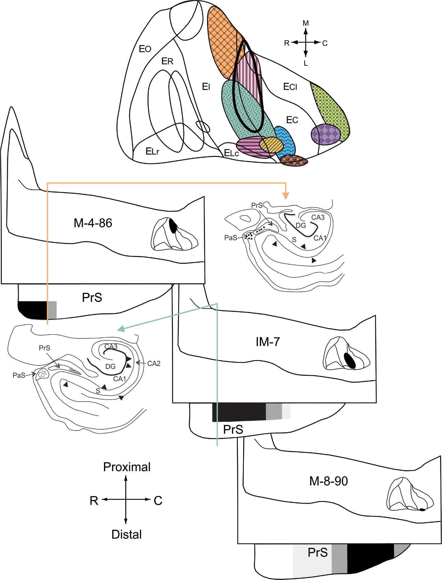
Illustration of the topographic organization of presubicular projections to the entorhinal cortex. The locations and extents of entorhinal retrograde tracer injections that resulted in labeled cells in the presubiculum are indicated with different shading/color patterns on an unfolded two dimensional entorhinal map (top). Injections (located in rostral levels of the entorhinal cortex) that did not produce retrograde labeling in the presubiculum are indicated by outlines only (compare with Figure 3). Schematic representations (bottom) of the distributions and densities of retrogradely labeled cells in the presubiculum following three representative injections in the entorhinal cortex. The three entorhinal injections are located at approximately the same rostrocaudal level but differ with respect to their lateromedial position (see upper panel for locations of injections indicated by the shading/color patterns). The highest densities of retrogradely labeled cells were represented by black shading, intermediate densities by dark grey shading and low densities by light grey shading. White indicates regions in which no labeled cells were found. Cell counts were summed across sections that represented 10% of the total rostrocaudal extent of the presubiculum. Insets are two representative coronal sections taken at approximately the same rostrocaudal level (indicated by the color-coded arrows) showing the differential distribution of retrogradely labeled neurons in distal versus proximal presubiculum associated with a medial versus lateral position of the injection site (case M-4–86 vs. case IM-7) [Color figure can be viewed at wileyonlinelibrary.com]

In order to represent the overall distribution of fiber and terminal labeling in the entorhinal cortex resulting from the ³H-amino acid or PHA-L injections, drawings of the coronal sections through the entorhinal cortex were “unfolded” to construct a two-dimensional map. The method by which these unfolded maps are constructed has been described previously (Amaral et al., 1987; Suzuki & Amaral, 1996). An unfolded map of the CA1 field of the hippocampus and the subiculum, presubiculum and parasubiculum was made in a similar manner (Figure 1–see figure legend for additional information).

FIGURE 1.

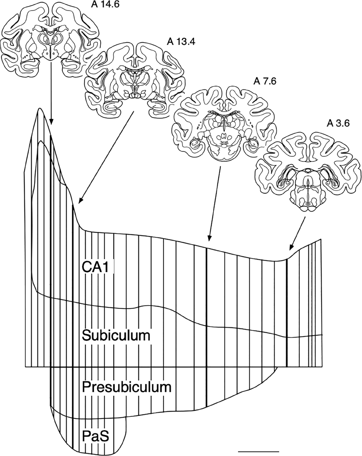
An “unfolded” two-dimensional map of CA1, subiculum, presubiculum and parasubiculum (PaS). The border between the subiculum and the presubiculum was used to align the sections and the linear extent of each field was represented as a straight line perpendicular to this line. Four representative sections, from rostral (A 14.6) to caudal (A 3.6) are presented for orientation (Nissl-stained sections from approximately these levels are illustrated in Figure 2). In order to unfold the most rostral or uncal portion of CA1 and the subiculum, the length of the uncal portion of each field has been merged with that of the corresponding part in the body of the hippocampus from the same section. This eliminates the intervening portion of CA3 and CA2 from the illustration. The map is constructed from 34 representative sections that are distributed throughout the rostrocaudal extent of the hippocampal formation. More sections were used at extreme rostral and caudal levels where the hippocampal fields change more rapidly

Half tone photomicrographs used for Figures 2, 11, and 16 were initially acquired using standard 35 mm or 4 × 5 in. format photomicrography systems. For Figure 2, 4 × 55 negatives were scanned using a UMAX flatbed scanner and imported into Adobe Photoshop (v. 4.0). The images were adjusted for optimal contrast, and lettering was added. The darkfield images used in Figures 11 and 16 were first printed and the prints scanned. Artifacts surrounding the sections were eliminated and the images were adjusted for contrast and brightness. Regional or laminar borders were traced from adjacent Nissl-stained sections, the drawings were scanned, and the borders were ultimately superimposed on the base print in Adobe Photoshop.

FIGURE 2.

Photomicrographs of four coronal Nissl-stained sections located at different rostrocaudal levels of the hippocampal formation. Sections are arranged from rostral (a) to caudal (d). The various boundaries between divisions of the hippocampal formation are indicated. The photomicrographs in Panels a–d approximately correspond to the levels of the four sections indicated in Figure 1 (A14.6, 13.4, 7.6, and 3.6 respectively). Scale bar equals 1 mm

FIGURE 11.

Darkfield photomicrographs of PHA-L labeling in the entorhinal cortex resulting from the injections in CA1 illustrated in Figure 9. (a) Labeling in the rostral entorhinal cortex following an injection in the distal portion of CA1 (case M-30–92); (b) Labeling in the caudal entorhinal cortex following a PHA-L injection located in the proximal portion of CA1 (case M-5–89). Scale bar equals 2 mm

FIGURE 16.

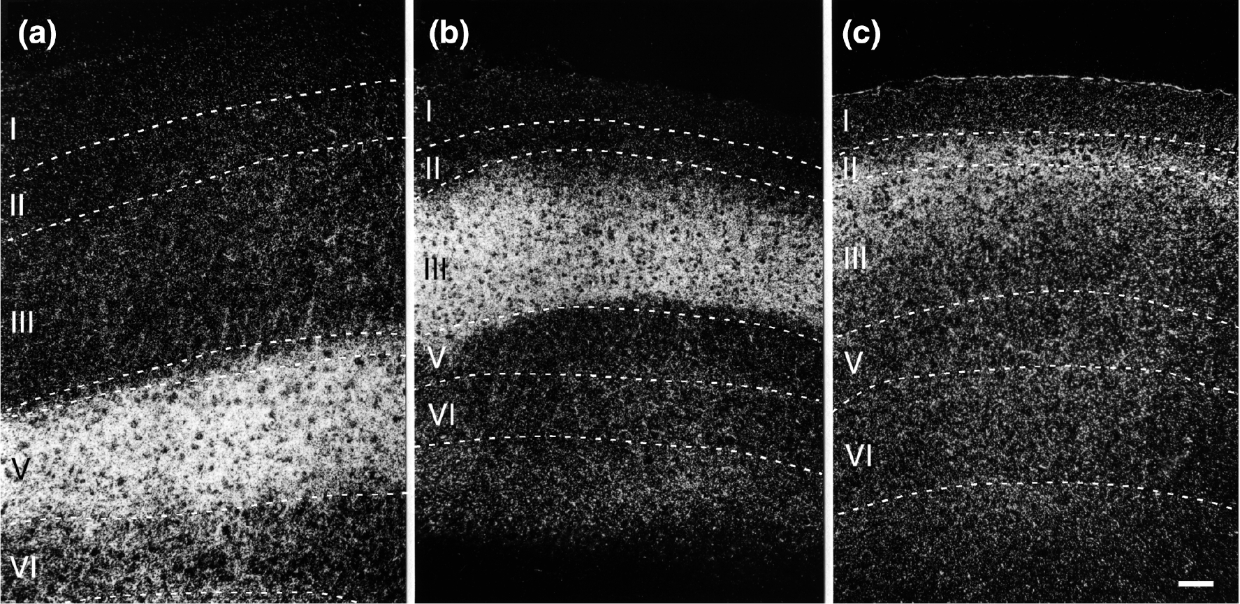
Darkfield photomicrographs illustrating the laminar organization of anterograde labeling in the ipsilateral entorhinal cortex following ³H-amino acid injections in the subiculum (a; case M-5–84), the presubiculum (b; case DM-16), and the parasubiculum (c; case DM-17). The pattern of dense labeling in Layer V resulting from subicular injections (a) is similar to that produced following CA1 injections (see Figure 11). The labeling resulting from injections in the presubiculum (b) is most dense in Layer III. Injections in the parasubiculum produce dense labeling in Layers II and III of the entorhinal cortex (c). Scale bar equals 100 μm

3 |. RESULTS

3.1 |. Nomenclature

The hippocampal region comprises the dentate gyrus, the hippocampus, the subiculum, the presubiculum, the parasubiculum, and the entorhinal cortex. The cytoarchitectonic organization of the monkey hippocampal region has been described extensively (Kobayashi & Amaral, 1998; Pitkanen & Amaral, 1993) and the following is an abridged description of the nomenclature and subdivisions that are necessary for the interpretation of the results presented in this article. Nissl-stained photomicrographs of coronal sections through four rostrocaudal levels of the hippocampal region are shown in Figure 2.

The dentate gyrus is comprised of three layers (molecular layer, granule cell layer, and polymorphic layer) The hippocampus proper is divided into three distinct fields: CA3, CA2, and CA1. Fields CA3 and CA2 are characterized by large pyramidal cells which are located in a relatively compact principal cell layer. Field CA1 has smaller pyramidal cells in its principal cell layer which is substantially thicker than in CA2 and CA3.

The border of the CA1 field with the subiculum is quite oblique; the progressively thinner CA1 pyramidal cell layer actually extends over the initial portion of the subiculum. The pyramidal cell layer of the subiculum is slightly thicker than that of CA1. The border between the subiculum and CA1 is sometimes marked by a narrow, obliquely oriented cell-sparse zone in the pyramidal cell layer but this is often obscured by an increased density of small, darkly stained cells. Some authors (Lorente de Nó, 1934; D.L. Rosene & Van Hoesen, 1987) have given the name prosubiculum to this border region between CA1 and the subiculum. Recent studies in the mouse focusing on genetic profiling of neurons have shown that the subiculum actually may be much more complex (Bienkowski et al., 2018; Cembrowski et al., 2018). Since such data are not available yet in the primate, we opted to stay consistent with our previous reports on the entorhinal efferents to the hippocampus and did not give this region a special name. Rather we view it as an area where cells with typical CA1 characteristics (such as receiving a projection from CA3) overlap with cells that appear to be typical subicular cells.

The presubiculum and parasubiculum have a cell free Layer I and a densely superficial cellular layer, often referred to as Layer II or Layer II/III. There are scattered cells deep to this layer of the presubiculum and parasubiculum that are often included as deep layers of these regions. It is unclear in the monkey, however, whether these cells are associated with these regions or are instead an extension of the deep layers of the entorhinal cortex (Amaral et al., 1987).

The monkey entorhinal cortex has been divided into seven cytoarchitectonically distinct divisions (Amaral et al., 1987). Other than the most rostrally situated division, EO or olfactory division (which was so named because it is the only component of the monkey entorhinal cortex that receives a direct projection from the olfactory bulb), the other fields are named for their positions within the entorhinal cortex. These divisions are: ER, rostral division, EL, lateral division (subdivided into a rostral (ELr) and a caudal (ELc), EI, intermediate division, EC caudal division, and ECL caudal limiting division. The entorhinal cortex contains six layers. These include: Layer I, a cell poor layer beneath the pia; Layer II, a thin layer of darkly stained, modified pyramidal cells, generally referred to as stellate cells, which are sometimes grouped into islands; Layer III, a broad, densely packed cellular layer in which the cells tend to be organized in patches rostrally but that is more columnar caudally; Layer IV, a narrow cell free layer (the lamina dissecans) that is only clearly visible in EI; Layer V, a band of large pyramidal cells that can be subdivided into two superficial laminae (Va and Vb) with cells of different sizes and a deeper, largely acellular lamina (Layer Vc); and Layer VI, which is a relatively thick cellular layer that, at caudal levels, has the appearance of coiled rows of cells. It is important to point out that these seven subdivisions are based on cyto- and chemo-architecture as well as some hodological data (EO), but do not yet have very clear functional connotations. Recent studies seem to converge on a functionally defined divide into two areas, referred to as (rostro)lateral and (caudo)medial entorhinal cortex (for a recent review see Nilssen et al., 2019), which we will address in detail in the discussion.

In all fields, we use the term “superficial” to mean toward the pia (or hippocampal fissure). The long axis of the hippocampus is referred to as the rostrocaudal axis (equivalent to the temporoseptal or ventrodorsal axis in the rodent). The axis orthogonal to the rostrocaudal axis is the transverse axis. Within any particular field of the hippocampal formation, the portion closer to the dentate gyrus is said to be proximal and that closer to the rhinal sulcus is distal. Thus, the proximal border of CA1 is with CA2 and the distal border is with the subiculum. In the entorhinal cortex we will use a comparable rostrocaudal nomenclature and the axis orthogonal to that will be referred to as the mediolateral axis (Figure 3).

FIGURE 3.

Unfolded two-dimensional map of the entorhinal cortex illustrating the locations and extents of retrograde tracer injections (see Table 1 for a summary of the tracers that were used) [Color figure can be viewed at wileyonlinelibrary.com]

3.2 |. Projections of the hippocampus and subiculum to the entorhinal cortex: retrograde tracer experiments

Before beginning our description of hippocampal and subicular projections to the entorhinal cortex, it is important to point out that the retrograde and anterograde tracing experiments consistently indicated that neither the dentate gyrus nor the CA3/CA2 fields of the hippocampus project to the entorhinal cortex. Although the retrograde cases showed sparse neuronal labeling in some cases which we attribute to uptake by passing damaged fibers (Illert, Fritz, Aschoff, & Hollander, 1982; Sawchenko & Swanson, 1981), the PHA-L injections in CA3/CA2 (Table 1) never provided evidence of fibers to the entorhinal cortex. We should also note that in the presentation below, the organization of projections from CA1 and the subiculum are described together. The rationale for organizing the description in this way is that our previous studies of the perforant path projections indicated that the cells of origin of entorhinal projections to these fields were all located in Layer III of the entorhinal cortex. Moreover, the laminar and transverse distribution of entorhinal fibers was similar in the subiculum and CA1. As described below, the organization of the projections back to the entorhinal cortex can also be most easily appreciated if the two fields are described together.

A summary of the distribution of retrograde tracer injections in the entorhinal cortex is illustrated in Figure 3. All the major subdivisions of the entorhinal cortex were involved in one or more of these injections although most of the injections were not confined to a single division of the entorhinal cortex. All the injections illustrated in Figure 3 produced retrogradely labeled cells in CA1 and the subiculum. The distribution of retrogradely labeled cells in 4 representative experiments is plotted on a series of coronal sections in Figures 4, and 5, and on unfolded maps of the complete rostrocaudal and transverse extents of CA1 and subiculum in Figure 6. Retrogradely labeled cells were intermingled with unlabeled neurons, and no clustering was apparent. However, as described below we observed a marked topographical distribution of labeled neurons.

Following an anteromedially positioned injection, involving medial EO and anteromedial EI (IM-4), many retrogradely labeled cells were present in rostral levels of CA1 and subiculum, in particular at the border region of the two areas, i.e. in distal CA1 and proximal subiculum (Figure 4a,b). At more caudal levels, the numbers of labeled neurons dropped off substantially, though maintaining the same transverse position as seen at rostral levels (Figure 4c,d). Following this injection, no retrogradely labeled cells were present in the presubiculum or the parasubiculum. In contrast, an injection involving posteromedial EI and caudally adjacent EC (M-4–86), resulted in labeling in CA1, the subiculum as well as in the presubiculum and parasubiculum. Labeling in CA1 and the subiculum was only present rostrally and confined to proximal parts of CA1 and distal parts of the subiculum (Figure 4e,f,g most medial part). Following an injection centered laterally at the border between fields ER and EI (M-11–90 DY), retrogradely labeled neurons were seen in CA1 and the subiculum, but not in the presubiculum or parasubiculum. Many labeled neurons were present in CA1 and the subiculum throughout their rostrocaudal extents, and preferentially distributed along the border of the two fields, thus in distal CA1 and adjacent proximal subiculum (Figure 5a–d). A more caudally positioned injection, centered in the very lateral part of EC, and extending into the adjacent perirhinal cortex (M-8–90; Figure 5e–h) resulted in retrograde labeling of neurons in CA1, the subiculum as well as in the presubiculum and the parasubiculum. Labeling is present along most of the rostrocaudal extent, though with a preference for the caudal parts, and avoiding the anteromedial levels of the head of the hippocampus. The labeled neurons in CA1 were preferentially found in the distal half, although the proximal part of CA1 also consistently showed labeled neurons. Labeled neurons in the subiculum were sparse and in more caudal levels preferentially present in the distal part (Figure 5h).

In recent years, it has been emphasized that CA1 and subiculum show connectional differentiation of pyramidal cells along the deep-to-superficial axis of the cell layer (for a comparative review on CA1 see Slomianka, Amrein, Knuesel, Sørensen, & Wolfer, 2011). In the monkey, projections to orbitofrontal and medial-prefrontal areas preferentially originate from deeper neurons (Barbas & Blatt, 1995; Cavada, Company, Tejedor, Cruz-Rizzolo, & Reinoso-Suarez, 2000), whereas projections to the perirhinal cortex originate mainly from more superficially located neurons (Ichinohe & Rockland, 2005). Comparable observations in the subiculum have been reported in rodents as well (Bienkowski et al., 2018; Cembrowski, Wang, et al., 2018; Ishizuka, 2001). While we did not carry out a detailed analysis of the radial organization of the retrogradely labeled cells, our observations appear to be in general agreement with the organization described above.

The topographical distribution of labeled neurons in CA1 and subiculum can be best appreciated in the unfolded representations (Figure 6). The regions with the highest density of labeled cells are indicated with black shading, with intermediate density by dark grey shading and with a low density of labeled cells by light grey shading. Several organizational features can be appreciated from these maps. First, essentially all rostrocaudal and transverse portions of CA1 and the subiculum demonstrated retrogradely labeled cells in one or the other of the various experiments. Second, consistent with the topographic organization of the perforant path, injections located medially in the entorhinal cortex (IM-4 and M-4–86) led to labeled cells in rostral levels of CA1 and the subiculum (see also Figure 4). In contrast, injections situated in the lateral portion of the entorhinal cortex (M-11–90 DY and M-8–90) tended to label cells located more caudally in CA1 and the subiculum (see also Figure 5). Third, comparing injections located at the same mediolateral position in the entorhinal cortex showed that the more rostral injections (IM-4 and M-11–90 DY) resulted in more labeled cells near the CA1/subiculum border, whereas more caudally situated injections (M-4–86 and M-8–90) resulted in more labeled cells situated distally in the subiculum and more proximally in CA1. The latter pattern is particularly clear in the case of M-4–86 compared to IM-4 (see also Figure 4a,e), whereas in M-8–90, the topographic organization might be obscured due to involvement of the perirhinal cortex in the injection site (the perirhinal cortex has been reported to project to the region around the border between CA1 and the subiculum Suzuki & Amaral, 1990). Moreover, the patterns may be obscured because retrogradely transported tracers are known to be taken up by injured fibers of passage (Illert et al., 1982; Sawchenko & Swanson, 1981). For these reasons, the rostrocaudal and the transverse gradients of the CA1/subiculum projections to the entorhinal cortex were more easily and convincingly appreciated in the anterograde tracer experiments.

3.3 |. Projections of the hippocampus and subiculum to the entorhinal cortex: anterograde tracer experiments

The locations and sizes of representative ³H-amino acid and PHA-L injections are illustrated on an unfolded map of CA1 and subiculum (Figure 7). In all cases, we observed labeling in the ipsilateral entorhinal cortex, mainly in the deeper layers. No labeling was observed contralaterally. The distribution and density of anterogradely transported label in nine of these experiments is plotted on the unfolded maps of the entorhinal cortex that comprise Figure 8. The unfolded maps are arranged so that those representing rostral injections are to the left and more caudal injections are to the right; injections in the proximal part of CA1 are at the top of the illustration, those on the CA1/subiculum border are in the middle (except for experiment MF-1 which has an injection in the proximal half of CA1) and those positioned distally in the subiculum are at the bottom.

FIGURE 7.

Unfolded two-dimensional map of CA1 and the subiculum that illustrates the locations and extents of representative anterograde tracer injections along the rostrocaudal and transverse (proximodistal) axes. All injections were of 3H-amino acids except for M-21–91, M-5–89, and M-30–92 which were PHA-L injections (see Table 1 for further details) [Color figure can be viewed at wileyonlinelibrary.com]

FIGURE 8.

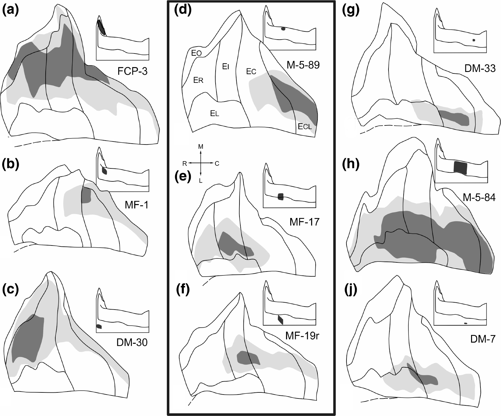
Unfolded two dimensional maps of the entorhinal cortex which illustrate the distribution and relative densities of anterograde labeling following nine representative injections of CA1 or the subiculum. The injection sites are shown in Figure 7. On each map, the density of anterogradely labeled fibers and terminals has been qualitatively represented as either high (dark shading) or moderate to low (light shading). White indicates regions where few if any anterogradely transported tracer was observed. The position of each of the nine maps in the illustration corresponds to the relative positions of the injection sites. The maps at left represent injections into the rostral CA1/subiculum and those at right represent injections at caudal levels of the CA1/subiculum. The middle row of maps represents injections located at about mid rostrocaudal levels. For rostrocaudal comparisons, a–c should be compared with d–f and with g–j. Note that a rostral-to-caudal shift of the injection site results in a medial-to-lateral shift of the terminal field. The unfolded maps in the central, boxed area provide a clear comparison of the distribution of labeling following injections that differ in their transverse locations (d-f respectively; see also Figure 9). Injections of either the proximal CA1 (d) or the distal subiculum (f) lead to labeling in the caudal portion of the entorhinal cortex whereas an injection located on the CA1/subiculum border (e) leads to labeling more rostrally in the entorhinal cortex

Taken together, the various experiments demonstrate that all rostrocaudal and mediolateral portions of the entorhinal cortex receive a topographically organized projection from CA1 and the subiculum. Injections located rostrally in the CA1 or subiculum (FCP-3, MF-1 and DM-30; Figure 8a–c) led to fiber and terminal labeling situated in the medial portion of the entorhinal cortex whereas more caudally situated injection sites (DM-33, M-5–84, and DM-7; Figure 8g–j) led to labeling that was focused in the lateral aspect of the entorhinal cortex. By investigating injections located at roughly the same intermediate rostrocaudal level in CA1 and the subiculum (M-5–89, MF-17, and MF-19r), the relationship of the transverse location of the injection site to the pattern of labeling becomes apparent. The terminal fields of these three injections together form a band extending from the rostral to the caudal poles of the mid mediolateral portion of the entorhinal cortex (Figure 8d–f). If the injection was located either proximally in CA1 (M-5–89) or distally in the subiculum (MF-19r), the labeling was distributed to the caudal portion of the band. In contrast, if the injection was located on the CA1/subiculum border, (MF-17) the projection terminated mainly in the rostral half of the band. When the injection was very large and covered much of the full transverse extent of CA1 or the subiculum (such as in experiment M-5–84), the band of labeling extended along the full rostrocaudal extent of the entorhinal cortex.

The transverse organization of the CA1 projection is perhaps most clearly appreciated in the comparison of two experiments in which PHA-L was injected at the same rostrocaudal level in either the proximal (M-5–89) or distal (M-30–92) extremes of CA1 (Figures 9 and 10a,b). Labeling from both injections was confined to the same mediolateral region within the entorhinal cortex. The proximal injection, resulted in labeling that began in the caudal half of EC and was densest in ECL. The distal injection, in contrast, resulted in labeling that was densest in ER and EI and tapered off in EC. In other words, there was little or no overlap in the areas innervated by the two populations of CA1 pyramidal cells located at approximately the same rostrocaudal level of the hippocampus.

FIGURE 9.

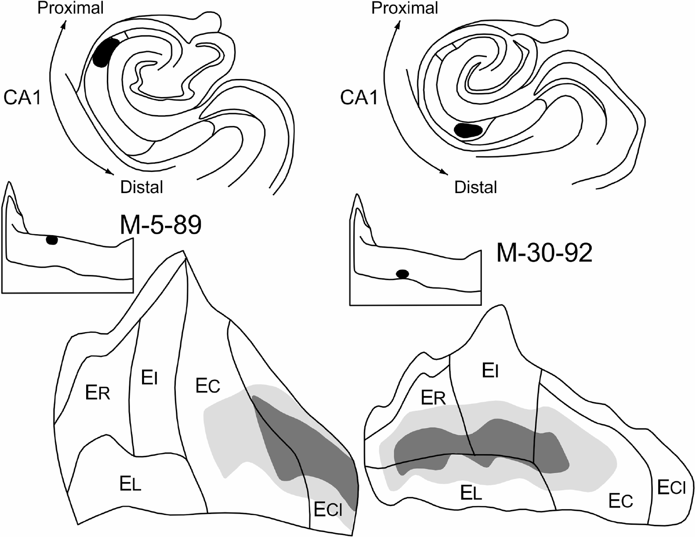
Comparison of the distribution of labeled fibers and terminals in the entorhinal cortex resulting from PHA-L injections located either proximally or distally in the CA1 field of the hippocampus. The line drawings of coronal sections at the top illustrate the size and location of the PHA-L injections. The distributions and relative densities of anterogradely transported label from each of these injections is represented on the unfolded two-dimensional maps of the entorhinal cortex located at the bottom of the illustration. A shift of the injection site from proximal CA1 (M-5–89; left side) to distal CA1 (M-30–92; right side) results in a corresponding shift of the terminal field in the entorhinal cortex from caudal to rostral. Since these injections are at the same rostrocaudal level of CA1, there is no change in the position of the terminal field along the lateral to medial axis of the entorhinal cortex

The pattern of fiber and terminal labeling resulting from the PHA-L injections described above is shown photomicrographically in Figure 11. The densest projection in both cases was to Layer V. As can be seen in Figure 11a, the distal CA1 injection led to strong labeling in rostral EI. The proximal CA1 injection, in contrast, led to strong labeling in EC (Figure 11b). At these levels, dense terminal labeling was seen in Layer V, particularly in Va and Vb, with almost no labeling, except for some passing fibers in Vc. Layer VI had a mixture of labeled fibers of passage, as well as some branching, terminating fibers. Also, some branching, varicose labeled fibers ascended from Layer V into Layers III and I. Following injections in the subiculum, such as case M-5–84, a similar laminar pattern was observed (Figure 16a).

3.4 |. Projections from the presubiculum to the entorhinal cortex: retrograde tracer studies

Only retrograde tracer injections that involved caudal entorhinal cortex (caudal EI, EC, ECL, or ELc resulted in retrograde labeling in the presubiculum (Figures 4, 5, and 12). Injections in rostral EI (IM-4 and M-II-90 DY; Figures 4a–d and 5a–d) and even relatively large injections of retrograde tracers in ER (such as IM-6 or IM-8; Figures 3 and 12) did not lead to presubicular labeling. Injections of the medial portion of the caudal entorhinal cortex, involving caudal EI and adjacent EC (M-4–86; Figures 4e–g, 12) resulted in retrogradely labeled cells through rostral levels of the presubiculum, whereas injections involving the lateral portion of the entorhinal cortex (M-8–90) led to an increase in the number of retrograde labeled neurons at more caudal levels of the presubiculum (Figures 5e–g, 12). Comparison of the distribution patterns of retrogradely labeled cells in cases IM-7 and M-4–86 (Figure 12) suggested that, as in the rat (Caballero-Bleda & Witter, 1993), there may also be a transverse component to the organization of the presubicular projections. Proximal and distal portions of the presubiculum may preferentially innervate lateral and medial portions, respectively, of the entorhinal cortex.

3.5 |. Projections from the presubiculum to the entorhinal cortex: anterograde tracer studies

The anterograde tracer experiments confirmed and extended the observations made from the retrograde material. Regardless of the rostrocaudal or mediolateral position of the presubicular injection, there was little or no labeling of ER, EO, or the rostral part of EL (Figure 13). Despite the rostrocaudally more constrained terminal area in the entorhinal cortex, some of the same aspects of the topographic organization observed for the CA1/subiculum projections were also observed for the presubiculum projection.

FIGURE 13.

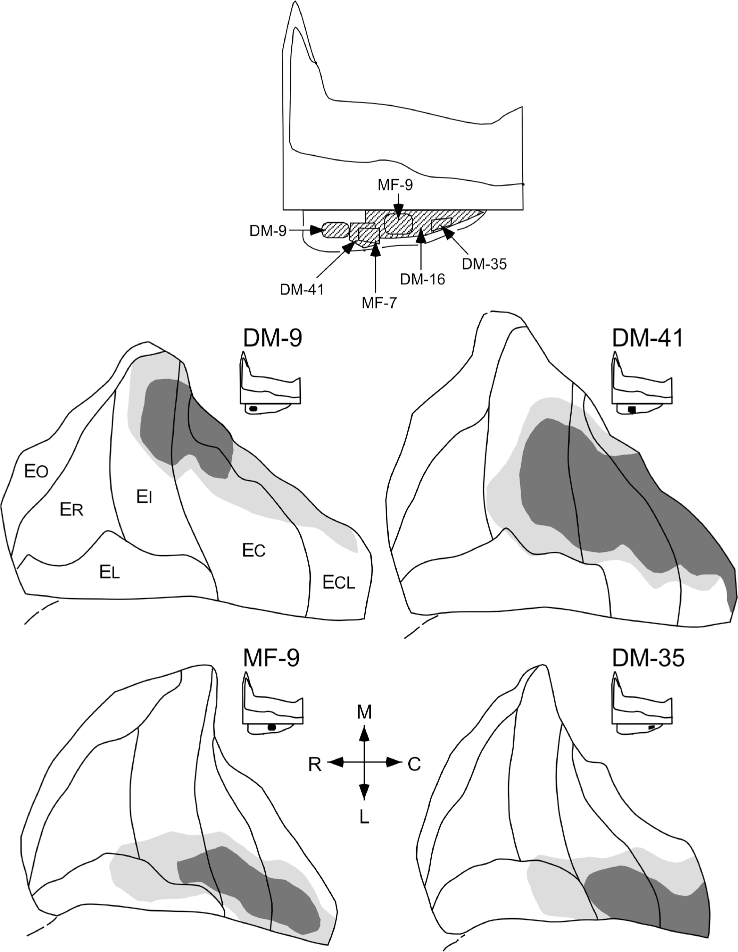
Unfolded two-dimensional maps of the entorhinal cortex that demonstrate the distribution and relative densities of anterograde labeling following ³H-amino acid injections at four different positions along the rostrocaudal axis of the presubiculum. The density of anterograde labeling in the entorhinal cortex is represented qualitatively as either high (dark shading) or low to moderate (light shading). White represents areas with little or no anterogradely transported label. The locations of presubicular injection sites are represented on an unfolded map (bottom)

Injections of rostral levels of the presubiculum (DM-9 and DM-41) resulted in dense labeling of the medial portion of the entorhinal cortex (Figure 13). Presubicular injections at progressively more caudal levels (MF-9; injection site shown in Figure 10c; and DM-35) resulted in progressively more laterally situated terminal fields in the entorhinal cortex. An additional unfolded map of an experiment with a presubicular injection is illustrated in the top portion of Figure 14. In this case (DM-16), three injections of ³H-amino acids were made at positions that encompassed the caudal two-thirds of the presubiculum (Figure 13). As indicated in the unfolded entorhinal map shown in Figure 14, despite the large size of this injection there was essentially no labeling of the rostral entorhinal cortex (ER, EO, and ELr). Moreover, since the rostral portion of the presubiculum was not involved by the injection, the most medial portion of the caudal entorhinal cortex was unlabeled. Due to the small number of injections involving the presubiculum, the anterograde material provided no clarification of whether a transverse organization exists in the presubicular projections to the entorhinal cortex, that is, whether medial portions of the presubiculum might project to different regions of the entorhinal cortex than lateral portions of the presubiculum.

FIGURE 14.

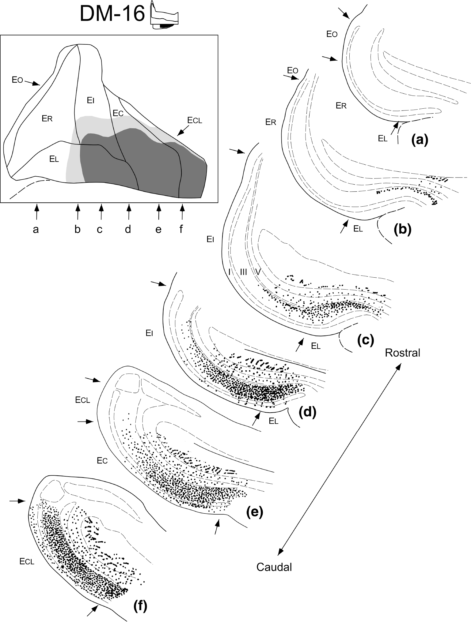
Illustration of the extent and laminar organization of presubicular projections to the entorhinal cortex. This illustration represents data from experiment DM-16 in which three injections of ³H-amino acids involved the caudal two-thirds of the presubiculum (inset and also see Figure 13 for location of injection site). The unfolded map at top left shows the overall distribution of labeled fibers and terminals within the entorhinal cortex. The terminal labeling is confined to caudal portions of the entorhinal cortex. The line drawings at the right show representative coronal sections arranged from rostral (a) to caudal (f) through the entorhinal cortex (the approximate locations of these sections are indicated with the corresponding letters on the unfolded map). The density of labeled fibers and terminals is represented on the coronal sections as dots and small line segments. Dashed lines represent layers of the entorhinal cortex (c)

The presubicular projection to the entorhinal cortex produced a dense terminal field which demonstrated a consistent pattern of laminar distribution (Figures 14 and 16). Terminal labeling was densest within Layer III but there was also substantial labeling in Layer II and in the superficial part of Layer I. Autoradiographic grains were also observed in Layers V and VI, but these often had the appearance of fibers of passage. The presubicular injections tended to result in a densely labeled restricted area in the entorhinal cortex with a surrounding region of progressively sparser fiber and terminal labeling (Figures 13 and 14). The location of the terminal field tended to be deeper at rostral levels (confined usually to the deep portion of Layer III) and to spread throughout Layer III and into Layers II and I at more caudal levels (compare Figure 14c with e or f). The projections from the presubiculum are bilateral and, although the contralateral projection appears marginally weaker than the ipsilateral one, the laminar distribution is similar on both sides.

3.6 |. Projections from the parasubiculum to the entorhinal cortex: retrograde and anterograde tracing experiments

All of the retrograde tracer injections in the entorhinal cortex that gave rise to labeling in the presubiculum also resulted in labeled cells in the parasubiculum. Labeled cells were observed at rostral levels of the parasubiculum when the injections were situated medially in the entorhinal cortex (M-4–86; Figure 4g) and were more numerous caudally when the injection was located laterally in the entorhinal cortex (M-8–90; Figure 5g).

Anterograde tracing experiments confirmed the impression from the retrograde studies that the parasubiculum projected to the same regions as the presubiculum. Fibers from the parasubiculum appeared to terminate in Layers III and II of the entorhinal cortex (Figure 15). The parasubiculum has a denser projection to Layer II at caudal levels (Figures 15e,f and 16c). At progressively more rostral levels in the entorhinal cortex, the labeling in Layer III became more prominent (Figure 15b,c). In contrast to the projections from the presubiculum, which distributed bilaterally to the entorhinal cortex, the contralateral parasubicular projections appeared to be very weak or even absent in some cases.

FIGURE 15.

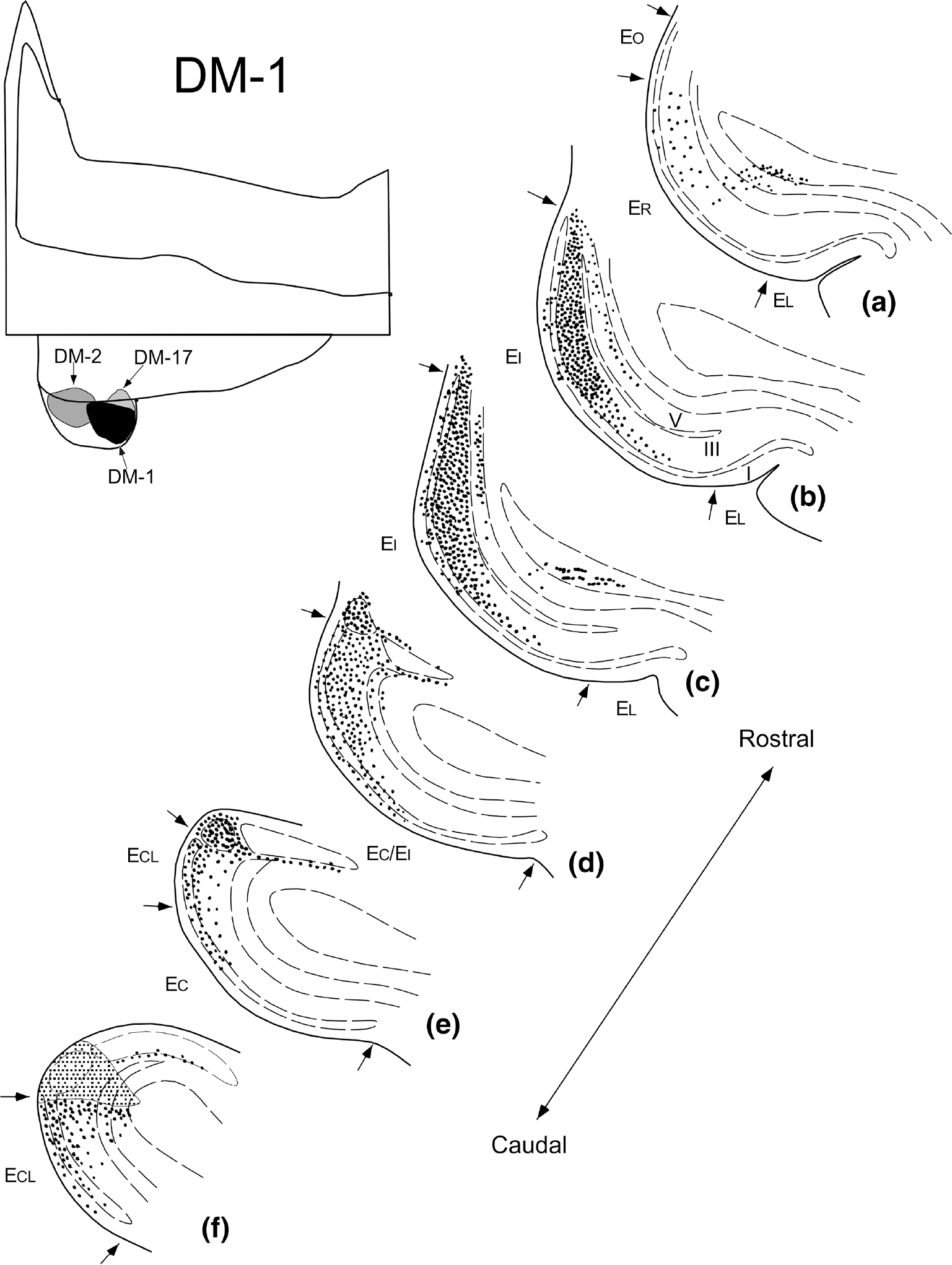
Illustration of the extent and laminar organization of parasubicular projections to the entorhinal cortex. This illustration represents data from experiment DM-1 in which an injection of ³H-amino acids involved the caudal half of the parasubiculum. The unfolded map at the top left shows the location of parasubicular injections analyzed for this study. The line drawings at the right show representative coronal sections arranged from rostral (a) to caudal (f) through the entorhinal cortex. The density of labeled fibers and terminals is represented on the coronal sections as dots and small line segments. Dashed lines represent layers of the entorhinal cortex (b). The injection site is illustrated as a shaded area in Panel f

4 |. DISCUSSION

4.1 |. Origin of the hippocampal projections to the entorhinal cortex

It is clear from both the retrograde and anterograde data described here that hippocampal projections to the entorhinal cortex originate exclusively in field CA1 of the hippocampus and in the subiculum, presubiculum and parasubiculum. The dentate gyrus and fields CA3/CA2 do not project to the entorhinal cortex. These observations are in agreement with those of Saunders and Rosene (1988) in the rhesus monkey. (Hjorth-Simonsen, 1973; Swanson & Cowan, 1977; Swanson, Sawchenko, & Cowan, 1981). Similar observations have been reported in the guinea pig (Sorensen & Shipley, 1979), the rat (Amaral & Witter, 1989; Beckstead, 1978; Ishizuka, Weber, & Amaral, 1990), and the cat (Room & Groenewegen, 1986b; van Groen, van Haren, Witter, & Groenewegen, 1986). With the exception of a recent report in rodents (Rowland et al., 2013) and in the cat (Ino et al., 2001) that CA2 projects to Layer II of the medial entorhinal cortex, all other reports in rodents are in line with the conclusion that hippocampal projections exclusively originate in CA1 and the subiculum.

4.2 |. Projections from CA1 and the subiculum

All parts of CA1 and the subiculum contribute to projections to the ipsilateral entorhinal cortex and all parts of the entorhinal cortex are innervated by CA1 and subicular inputs. These projections terminate most densely in Layer V of the entorhinal cortex, although weaker projections reach Layers III and I. Comparable observations have been reported in earlier studies in the rhesus monkey (D. L. Rosene & Van Hoesen, 1977; Saunders & Rosene, 1988), rat (Cenquizca & Swanson, 2007; Kloosterman, Witter, & Van Haeften, 2003; Köhler, 1985; Swanson & Cowan, 1977; Swanson, Wyss, & Cowan, 1978; van Haeften, Jorritsma-Byham, & Witter, 1995), guinea pig (Sorensen & Shipley, 1979), and cat (van Groen et al., 1986; Witter, Room, Groenewegen, & Lohman, 1986).

4.3 |. Projections from presubiculum and parasubiculum

As demonstrated previously in the monkey (Amaral, Insausti, & Cowan, 1984), and in line with observations in the rat and guinea pig (Caballero-Bleda & Witter, 1993; Shipley, 1974, 1975; van Haeften et al., 1997), the presubicular projections to the entorhinal cortex are bilateral, whereas the projections from the parasubiculum are almost exclusively ipsilateral. (Amaral et al., 1984)

Regarding the laminar distribution of pre- and parasubicular projections, the data are consistent across several species (Caballero-Bleda & Witter, 1993; Köhler, 1985; Shipley, 1975; Swanson & Cowan, 1977; van Groen & Wyss, 1990a, 1990b). The presubiculum in the monkey projects mainly to Layers III and to the deep half of Layer I, with weaker projections to Layers II and V, in line with previous reports (Saunders & Rosene, 1988). The parasubiculum also projects to Layer III, especially at rostral levels of the terminal field, but tends to project more strongly to Layer II than the presubiculum

4.4 |. Topographical organization

A major contribution of the current study is in the definition of the topographic organization of the hippocampal projections to the entorhinal cortex. We previously demonstrated (Witter & Amaral, 1991; Witter, Van Hoesen, & Amaral, 1989) that the perforant path projections to the dentate gyrus, hippocampus, and subiculum were organized in a distinctive topographic fashion. In the current study, we sought to determine whether the return projections to the entorhinal cortex followed the perforant path topography. In other words, would a region of the entorhinal cortex that originates a projection to a particular rostrocaudal or transverse portion of the hippocampus or subiculum receive a return projection from the same part of these fields? The current study allows this question to be answered in the affirmative. We conclude that the hippocampal projections to the entorhinal cortex are organized in a fashion that is remarkably consistent with the perforant path topography, that is, the return projections are spatially in register with the perforant path projections.

The major features of the topography of entorhinal inputs and outputs with the other hippocampal fields are summarized in Figure 17. The perforant path projection is organized such that neurons situated laterally in the entorhinal cortex, that is, located close to the rhinal fissure, project to caudal levels of the hippocampal formation and progressively more medially situated cells project to more rostral levels of the hippocampal formation. In the current study, we found that neurons located at caudal levels of CA1 and the subiculum project to lateral portions of the entorhinal cortex and more rostrally situated neurons in these fields project to more medially situated portions of the entorhinal cortex.

FIGURE 17.

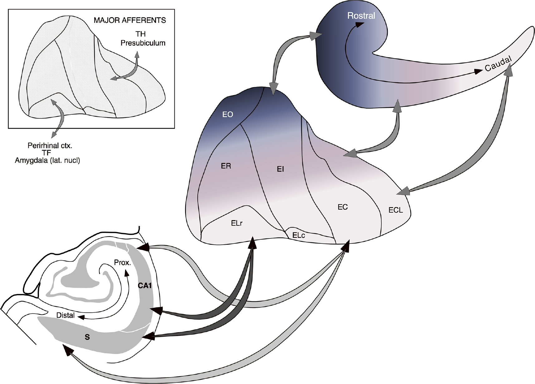
Summary diagram illustrating the major topographic features of entorhinal-hippocampal interconnectivity. The mediolateral organization of entorhinal-hippocampal interconnections is portrayed by the arrows running from the unfolded map of the entorhinal cortex located in the middle of the illustration toward the schematic hippocampus at top right. A rostrocaudally oriented band of entorhinal cortex located medially (blue shading) projects to rostral levels of the hippocampus and progressively more laterally situated bands of the entorhinal cortex (magenta to lighter shading) project to more caudal levels of the hippocampus. The relationship between the transverse (proximodistal) location of cells in CA1 and the subiculum and rostrocaudal levels of the entorhinal cortex is illustrated by the arrows extending toward the coronal section of the hippocampus/subiculum at lower left. Cells located at the border of the CA1 and subiculum receive inputs from and contribute inputs to the rostral portion of the entorhinal cortex. Cells located proximally in CA1 and distally in the subiculum receive inputs from and contribute inputs to caudal portions of the entorhinal cortex. The inset at top left indicates that inputs to the entorhinal cortex from the amygdala, the perirhinal cortex and area TF are preferentially directed to rostral levels, whereas inputs from the presubiculum and area TH are directed preferentially to caudal levels of the entorhinal cortex [Color figure can be viewed at wileyonlinelibrary.com]

The reciprocity of the connections was even more strikingly apparent when the transverse organization of the CA1/subiculum connections was evaluated (Figure 17). In our previous studies, we found that rostrally situated entorhinal cells project to the region at the CA1/subiculum border, that is, distal CA1 and proximal subiculum and more caudally situated cells project to more proximal portions of CA1 (closer to CA2) and more distal portions of the subiculum (closer to the presubiculum). In other words, CA1 or subicular neurons located at the same rostrocaudal level receive inputs from different portions of the entorhinal cortex depending on their transverse location. Those nearer the CA1/subiculum border are innervated from rostral levels of the entorhinal cortex, whereas those nearer the CA2 or presubicular border are innervated by caudal levels of the entorhinal cortex. In the current study, we found that the reverse was also true. At any particular rostrocaudal level of the hippocampal formation, neurons located in distal CA1 and proximal subiculum project to rostral levels of the entorhinal cortex, whereas cells located more proximally in CA1 and more distally in the subiculum project to more caudal levels of the entorhinal cortex.

While Saunders and Rosene (1988) did not explicitly describe the topographic organization of the CA1/subiculum interconnections with the entorhinal cortex, several of their figures nicely illustrated the organizational scheme described above. Their Figure 15, for example, depicts an experiment in which two retrograde tracers were injected at different rostrocaudal levels of the entorhinal cortex. One was rostrally and medially situated, the other was caudally and laterally situated. The rostral injection resulted in labeled cells at the CA1/subiculum border (due to its rostral position) primarily at rostral levels of the hippocampal formation (due to the medial location of the injection). The caudal injection resulted in retrogradely labeled cells in proximal CA1 and distal subiculum (due to its caudal location) which were situated mainly at caudal levels of the hippocampal formation (due to the lateral position in the entorhinal cortex. Since these investigators carried out their studies in M. mulatta (rhesus) monkeys and our studies were carried out in M. fascicularis monkeys, we conclude that the topographic organization is apparently consistent across macaque monkey species. In another study, Blatt and Rosene (1998) reported on the organization of projections from CA1 and the subiculum to temporal cortical regions and the entorhinal cortex. Based on their retrograde tracing studies, they conclude that projections to the entorhinal cortex only show a rostrocaudal gradient and that no transverse organization is present. As we have described in the current article, anterograde tracers such as PHA-L, which do not suffer from a fiber of passage problem, demonstrate a clear transverse organization of the CA1/subicular projections to the entorhinal cortex.

4.5 |. Implications of hippocampal-entorhinal connectivity

While a detailed evaluation of the implications of the topographic organization of the entorhinal-hippocampal interconnections must await further information concerning the topography of entorhinal afferents and associational connections within the entorhinal cortex, available data provide the basis for some comments (Figure 17).

4.5.1 |. Relationship between cytoarchitectonic subdivisions in EC and connectivity

A major observation is that while the full rostrocaudal extent of the presubiculum gave rise to an entorhinal projection, the terminal field included only the more caudal parts of the entorhinal cortex, i.e., areas EI _(caudal), ELC, EC, and ECL. In nonprimate species, the presubicular projections are also restricted to the more caudally located portions of the entorhinal area (Caballero-Bleda & Witter, 1993; Honda & Ishizuka, 2004; Honda & Shibata, 2017; Ino et al., 2001; Köhler, 1985; Room & Groenewegen, 1986b; Shipley, 1975; Swanson & Cowan, 1977; van Groen & Wyss, 1990a, 1990b). It is thus apparent that the distribution of presubicular inputs to Layer III does not adhere to the cytoarchitectonically defined seven subdivisions of the monkey EC. Likewise, an equally prominent input to Layer III from the lateral nucleus of the amygdala in the monkey is clearly confined to rostral levels of the entorhinal cortex (EO, ELR, and ER) (Pitkanen et al., 2002), and this is similar to what has been reported in nonprimate species (Pikkarainen, Rönkkö, Savander, Insausti, & Pitkänen, 1999; Pitkanen, Pikkarainen, Nurminen, & Ylinen, 2000; Room & Groenewegen, 1986a). The two inputs show almost complimentary distributions, thus dividing the entorhinal cortex into two hodologically defined subdivisions (see also Doan, Lagartos-Donate, Nilssen, Ohara, & Witter, 2019; Suzuki & Amaral, 1994b).

Traditionally, the entorhinal cortex has been considered to comprise two subdivisions, often referred to as Brodman’s Area 28 a and b, or lateral and medial entorhinal cortex, respectively. The use of area 28 has been largely discontinued, whereas the use of lateral and medial entorhinal cortex has become more commonly accepted, particularly in the rodent, where the two subdivisions can be easily differentiated cytoarchitectonically, and their projections to the dentate gyrus have different zones of termination in the molecular layer (Kjonigsen, Leergaard, Witter, & Bjaalie, 2011; Witter, 2007). However, more complex proposals have been published for several species, including the rat (Insausti, Herrero, & Witter, 1997; Krettek & Price, 1977b), the guinea pig (Uva, Gruschke, Biella, de Curtis, & Witter, 2004), and the cat (Krettek & Price, 1977a; Witter, Groenewegen, Lopes da Silva, & Lohman, 1989). A tripartite division into lateral, medial, and an intermediate transition entorhinal cortex has also been advocated (Blackstad, 1956; Lorente de Nó, 1933; Wyss, 1981). For monkeys, a variety of alternative divisions and nomenclatures have been proposed (Amaral et al., 1987 and references therein). For the present study, we used the scheme originally proposed by Amaral et al. (1987). For humans, an even larger variety of schemes have been proposed (see also Amaral et al., 1987; Insausti, Munoz-Lopez, Insausti, & Artacho-Perula, 2017; Insausti, Tunon, Sobreviela, Insausti, & Gonzalo, 1995; Krimer, Hyde, Herman, & Saunders, 1997; Stephan & Borgman, 1975; von Economo, 2009). More recently, functional studies in rodents provided strong support for a division into two areas, where neurons and networks in the medial entorhinal cortex seem to be strongly involved in allocentric representations of space, whereas the lateral entorhinal neurons and networks have become associated with a more egocentric coding of space and the passage of time (for a review see Nilssen et al., 2019). Since in nonprimate species, the presubicular input appears to clearly differentiate the medial from the lateral entorhinal areas, we suggest that the consistent distribution pattern of presubicular inputs to the entorhinal cortex in the monkey thus indicates that the monkey homologue of the nonprimate medial entorhinal area consists of caudal EI, ELC, EC, and ECL_. (Caballero-Bleda & Witter, 1993; Honda & Ishizuka, 2004; Honda & Shibata, 2017; Ino et al., 2001; Köhler, 1985; Nilssen et al., 2019; Room & Groenewegen, 1986b; Shipley, 1975; Swanson & Cowan, 1977; van Groen & Wyss, 1990a, 1990b).

It is of interest to note that the input from the retrosplenial cortex has also been proposed as a signature input to the medial entorhinal cortex in rodents and cats (Burwell & Amaral, 1998a; Jones & Witter, 2007; Room & Groenewegen, 1986b; Van Groen & Wyss, 2003). This input shows a spatial distribution that is similar to that of the presubiculum, except terminating preferentially in deeper layers of the entorhinal cortex. In the monkey, retrosplenial projections target caudal parts of EC, distributing mainly to EC and ECL with slightly weaker projections to caudal parts of EL and EI (Baleydier & Mauguiere, 1980; Insausti et al., 1987a; Kobayashi & Amaral, 2007; Morris, Petrides, & Pandya, 1999; Mufson & Pandya, 1984; Pandya, Van Hoesen, & Mesulam, 1981). Since in all species studied, the retrosplenial cortex and the presubiculum are also strongly interconnected, we propose that the two inputs combined might define the primate homologue of the medial entorhinal cortex (Doan et al., 2019; Nilssen et al., 2019). Our data support the proposition made in the latter studies (Doan et al., 2019; Nilssen et al., 2019) that the presubiculum and the retrosplenial cortex might be considered the better resting state connectivity indicators for the medial entorhinal cortex in the human rather than the parahippocampal/EC connectivity (Maass, Berron, Libby, Ranganath, & Duzel, 2015; Navarro Schroder, Haak, Zaragoza Jimenez, Beckmann, & Doeller, 2015). As argued above, inputs from the amygdala and the perirhinal cortex and parahippocampal area TF are suggested to be a defining feature of the primate lateral entorhinal cortex.

4.5.2 |. Topographical organization and reciprocity

Given the topography of the perforant path projections, the rostrocaudal segregation of these entorhinal inputs implies that at any particular rostrocaudal level of the hippocampus and subiculum, cells in different transverse positions would potentially be influenced by different types of information. Thus, cells at the CA1/subicular border, which receive perforant path fibers originating from rostral entorhinal cortex, would potentially be influenced by information arriving from the amygdala, perirhinal cortex, and area TF. Cells located more proximally in CA1 and more distally in the subiculum, in contrast, would potentially be more influenced by information arriving through the pre- and parasubiculum and area TH. Since CA1 as well as subicular neurons located at different transverse positions project to those rostrocaudal levels of the entorhinal cortex from which they receive their perforant path input, any functional segregation that is apparent within CA1 and subiculum would presumably be maintained through the projections back to the entorhinal cortex. The potential for segregation of processing is enhanced by the strict maintenance of this topography in the CA1-to subiculum projections (Naber, Lopes da Silva, & Witter, 2001; Tamamaki & Nojyo, 1995) and by the lack of substantial associational connections in CA1, at least in the rat (Amaral, Dolorfo, & Alvarez-Royo, 1991). Interestingly, in the subiculum a more developed associational network seems to exist (Fiske, Anstotz, Welty, & Maccaferri, 2020; Harris & Stewart, 2001; Harris, Witter, Weinstein, & Stewart, 2001), which might be reflected in the more complex neuronal firing properties in subiculum compared with CA1 (Lever, Burton, Jeewajee, O’Keefe, & Burgess, 2009; Sharp, 1997, 2006). Furthermore, since the entorhinal projections to the perirhinal and parahippocampal cortices are largely reciprocal (Suzuki & Amaral, 1994b), the segregation of information processing in the hippocampal-entorhinal circuitry may be sustained on the return projections to neocortex. Moreover, the direct projections from CA1 and the subiculum to the perirhinal and parahippocampal regions are mainly organized according to similar principles. Blatt and Rosene (1998) concluded that longitudinal strips of neurons located in the proximal part of CA1 and the distal part of the subiculum preferentially project to area TH, whereas neurons positioned in the border region between CA1 and the subiculum project to the perirhinal cortex and to area TF. These organizational features of the corticoentorhino-hippocampal projections largely parallel the situation in the rodent (for review see Doan et al., 2019; Nilssen et al., 2019).

Of course, the amount of segregation of these various inputs will depend on the extent of the association that takes place between rostral and caudal levels of the entorhinal cortex (Chrobak & Amaral, 2007; Dolorfo & Amaral, 1998; Ino, Kaneko, & Mizuno, 2000; Köhler, 1986, 1988; Witter et al., 1986). These rostrocaudal interactions seem to be mediated by neurons in Layer V and in superficial Layers II and III. In rodents, the latter includes the population of calbindin-expressing pyramidal neurons in deep Layer II (Ohara et al., 2019). Both in the monkey and the human entorhinal cortex, a similar population of calbindin-expressing neurons has been described, though the specific connectivity of these remains to be established (Naumann et al., 2016; Suzuki & Porteros, 2002). Additional association can take place through connections between the perirhinal and the parahippocampal cortices. Area TF of the parahippocampal cortex, for example, provides a prominent projection to the perirhinal cortex which is, however, largely unreciprocated (Suzuki & Amaral, 1994a). In the rat, postrhinal projections to perirhinal cortex are present that are stronger than the reciprocal ones (Burwell & Amaral, 1998b).

4.5.3 |. Functional nature of hippocampal and subicular inputs to entorhinal cortex

As discussed previously, the presubicular and parasubicular projections terminate mainly in Layers II and III, which are the sites of origin of the perforant path projections to the dentate gyrus and CA3 as well as to CA1 and the subiculum. The pre- and parasubiculum are considered to contribute extrinsic inputs to the entorhinal cortex and thus likely to the hippocampal formation. Although the pre- and parasubiculum receive weak inputs from CA1 and moderate inputs from the subiculum (present study; rat Cenquizca & Swanson, 2007; Honda et al., 1999; Köhler, 1985 but see in the rabbit Honda & Shibata, 2017), they are strongly interconnected both with the anterior nuclear complex and with the laterodorsal nucleus of the thalamus (van Groen & Wyss, 1990a, 1990b). Direct projections from these thalamic nuclei to the entorhinal cortex are sparse or absent (Insausti, Amaral, & Cowan, 1987b; Shibata, 1993; van Groen, Kadish, & Wyss, 1999; van Groen & Wyss, 1992). In addition, the monkey presubiculum receives a rather strong input from area 7 of the posterior parietal cortex (Seltzer & Van Hoesen, 1979) which projects only modestly to the entorhinal cortex and this has recently been reported to be true in the rat as well (Olsen, Ohara, Iijima, & Witter, 2017). Physiological data indicate that the inputs from the presubiculum and parasubiculum provide “head directional” information to the medial entorhinal cortex and this input has been shown to be relevant for the navigational potential of the animal, impacting spatially modulated neurons in the medial entorhinal cortex (Taube, 2007; Winter, Clark, & Taube, 2015). The amygdaloid projection, reaching more rostral portions of the entorhinal cortex may provide information concerning affective significance of events or stimuli (Kim et al., 1993).

While there are no data on the electrophysiology of the CA1/subicular projections to the monkey entorhinal cortex, these pathways have received substantial attention in rodents. From the early reports by Deadwyler, West, Cotman, and Lynch (1975) that stimulation of the CA3 field of the hippocampus produces field potentials in the ipsilateral entorhinal cortex that are accompanied by increases of extracellular unit firing, data have convincingly shown that projections from CA1/subiculum influence entorhinal networks through Layer V (Kloosterman, van Haeften, & Lopes da Silva, 2004; Kloosterman, Van Haeften, Witter, & Lopes Da Silva, 2003). Layer V is commonly subdivided into a Layers Va and Vb (Amaral et al., 1987; Boccara et al., 2015; Canto & Witter, 2012a, 2012b; Hamam, Amaral, & Alonso, 2002; Hamam, Kennedy, Alonso, & Amaral, 2000). In mice and rats, recent studies have pointed to a genetic differentiation, based on the expression pattern of transcription factors. Layer Va is characterized by a prominent expression of Etv1, whereas neurons in Layer Vb express Ctip2 and PtP4 (Ohara et al., 2018; Ramsden, Surmeli, McDonagh, & Nolan, 2015; Surmeli et al., 2016). This organization is consistent across the whole mediolateral and dorsoventral extent of the entorhinal cortex (Ohara et al., 2018). Layer Va cells are the major output neurons of the entorhinal cortex projecting to diverse cortical and subcortical structures (Kosel, Van Hoesen, & Rosene, 1982; Ohara et al., 2018; Surmeli et al., 2016; Swanson & Köhler, 1986; van Hoesen, 1982). Layer Vb neurons are the main recipients of the hippocampal and subicular return projections and project almost exclusively to superficial Layers II and III (Hamam et al., 2000; Hamam et al., 2002; Ohara et al., 2018; Surmeli et al., 2016). In the monkey, we lack data on such circuits, but we propose that similarly organized networks exist. In the rat it is known that the firing properties of grid cells, the signature spatially modulated neuron in Layer II of the medial entorhinal cortex, dramatically change when the hippocampus is pharmacologically silenced (Bonnevie et al., 2013). Since in the monkey medial entorhinal cortex grid-like neurons have also been reported (Wilming, Konig, Konig, & Buffalo, 2018), it would be of interest to know the effects of hippocampal silencing. Clearly, an understanding of the functional impact in primates of CA1 and subicular projections to the entorhinal cortex must await more detailed information concerning their cellular sites of termination and the organization of intrinsic connections between the deep and superficial layers of the entorhinal cortex.

Abbreviations:

29l, 29m

lateral and medial parts, respectively, of the retrosplenial cortex

35, 36

areas of the perirhinal cortex according to Brodmann (1909)

I - VI

layers of the entorhinal cortex

al

alveus

C

caudal

CA1, CA2, CA3

fields of the Hippocampus

DG

dentate gyrus

DY

Diamidino yellow (fluorescent retrograde tracer)

EC

entorhinal cortex

EC

caudal division of the entorhinal cortex

ECL

caudal limiting division of the entorhinal cortex

EI

intermediate division of the entorhinal cortex

ELR

rostrolateral division of the entorhinal cortex

ELC

caudolateral division of the entorhinal cortex

EO

olfactory division of the entorhinal cortex

ER

rostral division of the entorhinal cortex

FB

Fast blue (fluorescent retrograde tracer

gl

granule cell layer

L

lateral

M

medial

ml

molecular layer

ots

occipito-temporal sulcus

PaS

parasubiculum

pcl

pyramidal cell layer

pl

polymorphic layer

PHA-L

Phaseolus vulgaris leucoagglutinin (anterograde tracer), PrS presubiculum, R rostral

rs rhinal sulcus

S, subiculum

slm

stratum lacunosum-moleculare

so

stratum oriens

sr

stratum radiatum

TE, TF, TH

areas of the temporal lobe according to Bonin and Bailey (1947)

V

lateral ventricle

WGA-HRP

Wheatgerm agglutinin conjugated to horseradish peroxidase (retrograde tracer)

DATA AVAILABILITY STATEMENT

The experimental data will be made available on request to David G. Amaral.