Figure 5. Sensitivity of divergence time estimation to methodological decisions.

Between-group principal component analysis (bgPCA) was used to retrieve axes that separate chronograms based on the clock model (A), model of molecular evolution (B), and gene sampling strategy (C) employed. In the latter case, only the first two out of four bgPCA dimensions are shown. The inset shows the centroid for each loci sampling strategy, and the width of the lines connecting them are scaled to the inverse of the Euclidean distances that separates them (as a visual summary of overall similarity). The proportions of total variance explained are shown on the axis labels. The impact of the clock model is such that a bimodal distribution of chronograms can be seen even when bgPCA are built to discriminate based on other factors (as in C).

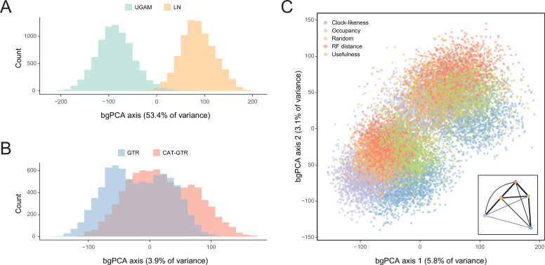
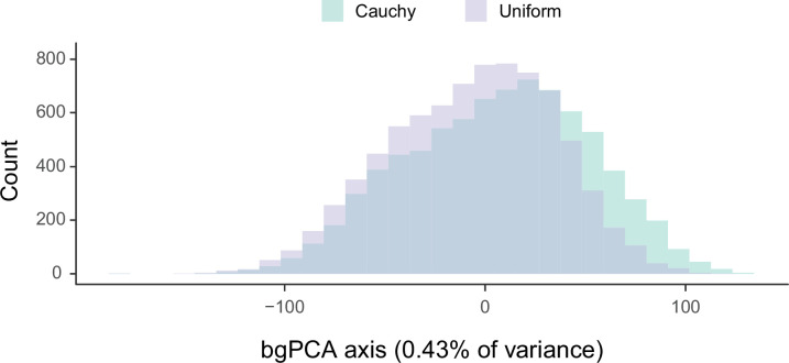
Figure 5—figure supplement 1. Sensitivity of divergence time estimation to the use of alternate prior distributions on calibrated nodes.

Between-group principal component analysis (bgPCA) was used to retrieve the axes of maximum discrimination between chronograms estimated by enforcing either uniform or Cauchy prior distributions. The proportion of total variance explained by this axis is shown on the label.

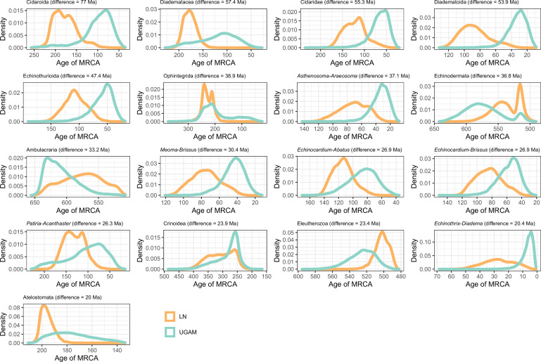
Figure 5—figure supplement 2. Distribution of posterior probabilities for node ages that show an average difference larger than 20 Myr depending on the choice of clock prior.

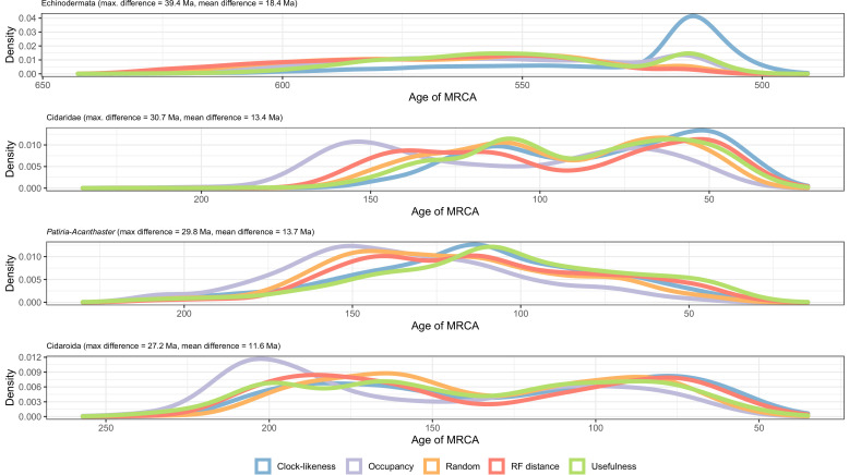
Figure 5—figure supplement 3. Distribution of posterior probabilities for node ages that show a maximum difference larger than 20 Myr depending on the gene sampling strategy.

The largest differences can be seen in the relatively younger ages of Ambulacraria and Echinodermata when using clock-like genes, and in the relatively older ages for some nodes within cidaroids and asteroids when using loci with high occupancy. Other sampling criteria largely agree on inferred node ages, as can also be seen in Figure 5C as short distances between their centroids in the chronospace.

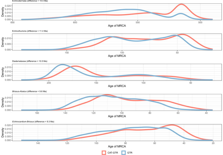
Figure 5—figure supplement 4. Distribution of posterior probabilities for node ages that are the most affected by the choice of model of molecular evolution.

No node showed average differences larger than 20 Myr, so those suffering the biggest changes are shown instead.

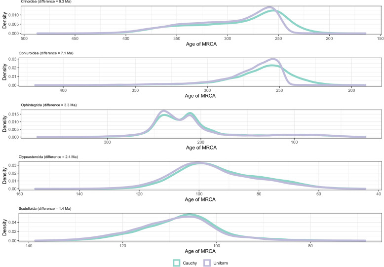
Figure 5—figure supplement 5. Distribution of posterior probabilities for node ages that are the most affected by the choice of prior distributions on calibrated nodes.

No node showed average differences larger than 20 Myr, so those suffering the biggest changes are shown instead.