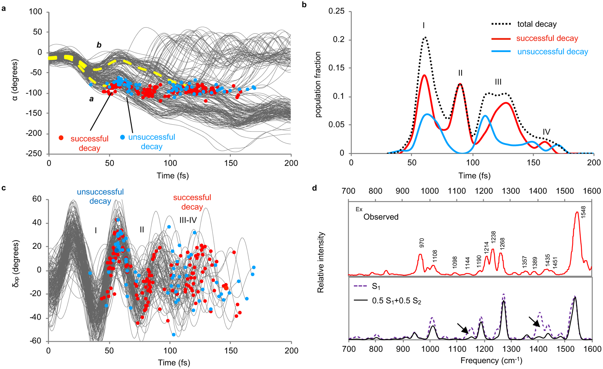
Fig. 2. Rh population dynamics.

(a) Time progression of α along a set of 200 trajectories simulating the S₁ population at room temperature and showing a motion initially coherent over the statistical ensemble²¹. The circles represent decays from S₁ to S₀. The splitting dashed curve in yellow serve as eye guidance tracing fast (a) and slow (b) decaying subpopulations. (b) Oscillatory character of the simulated S₁ population decay for both successful and unsuccessful trajectories. The four peaks have been resolved on the basis of the assumption that the standard deviation with respect to the average decay time of the peak has to be <10±1 fs. (c) Time progression of δ_op along the same trajectories. (d) Effect of the involvement of the S₂ state on the simulated resonance Raman spectrum. Top panel: Experimental spectrum.²² Bottom panel: Comparison between the resonance Raman spectra simulated using the S₁ gradient and using an equal mixture of S₁ and S₂ gradients according to the weighted-gradients method.²³ The arrows point at regions requiring both states for being correctly described.