Drinking Water, Fracking, and Infant Health

Abstract

This study assesses the health risks associated with drinking water contamination using variation in the timing and location of shale gas development (SGD). Our novel dataset, linking health and drinking water outcomes to shale gas activity through water sources, enables us to provide new estimates of the causal effects of water pollution on health and to isolate drinking water as a specific mechanism of exposure for SGD. We find consistent and robust evidence that drilling shale gas wells negatively impacts both drinking water quality and infant health. These results indicate large social costs of water pollution and provide impetus for re-visiting the regulation of public drinking water.

There is a well-established literature in economics that exposure to pollution has negative health consequences (Chay and Greenstone, 2003; Black et al., 2007; Currie and Walker, 2011; Sanders and Stoecker, 2015; Knittel et al., 2016; Schlenker and Walker, 2016; Isen et al., 2017; Hill, 2018; Deryugina et al., 2019). While work in this area has predominantly focused on the health impacts of air pollution, water pollution is a salient issue. Federal regulations such as the Safe Drinking Water Act and the Clean Water Act are motivated to control the health impacts of water pollution, and the recent water crisis in Flint, MI (Grossman and Slusky, 2019) has brought concerns about public drinking water quality to the forefront. Despite its relevance to policy and current environmental issues, the health effects of water pollution, especially at levels below regulatory thresholds, are not well-understood and the associated literature on causal impacts is thin.

This paper begins to fill this gap by assessing the infant health risks associated with drinking water contamination. Our identification strategy exploits the rapid expansion of shale gas development (SGD), commonly known as “fracking,” which has raised water-related health concerns for exposed populations (Muehlenbachs et al., 2015). We build a novel data set that links gas well activity to (1) infant health outcomes recorded from the universe of birth records in Pennsylvania, and (2) all ground water-based Community Water System (CWS) drinking water contaminant measurements. This is accomplished by using the exact geographic locations of maternal residences, gas wells, and public drinking water sources, as well as the dates of births, well bore activities, and water measurements. Combined, these data allow us to infer exposure to drinking water pollution from shale gas operations at both a high spatial and temporal resolution. We then use a difference-in-differences approach to estimate the impact of drilling near public water sources on public drinking water quality and the health of infants born to mothers who live in those systems.

Our paper makes two main contributions. First, we provide novel estimates on the causal impacts of water quality on health at mild levels as detected in developed countries. Isolating the health effects of water pollution has been difficult because data on water quality below thresholds of concern have been lacking. We innovate upon existing work by using the universe of public drinking water measurements to identify health effects below regulatory thresholds. The implications of our findings are especially important when viewed together with theory that predicts longer-term and inter-generational impacts on human capital accumulation and well-being from early-life exposures (Grossman, 1972, 1999; Almond and Currie, 2011; Cunha and Heckman, 2007; Almond et al., 2018) and recent empirical evidence on the importance of place for inter-generational mobility (Chetty and Hendren, 2018).

We are also the first paper to document that the pollution of public water supplies from fracking is affecting infant health. Our unique data on water source locations allow us to distinguish in utero exposure to SGD via water source proximity to gas wells drilled during gestation as opposed to exposure based solely on residential proximity. A finding that SGD operations have impacted water quality and health calls for regulation to internalize these consequences from an efficiency standpoint. The appropriate policy prescription to mitigate these impacts relies on identifying the mechanism of exposure.

We find consistent evidence that SGD affects both drinking water quality and birth outcomes. Drilling an additional gas well within a kilometer of ground water sources increases sampled SGD water chemicals by 1 percent and detection of regulated SGD chemicals by between 10 and 20 percent. The magnitude of this increase is large enough to surpass public health goals for these chemicals, but are too small to trigger a health based drinking water violation (reducing the likelihood that consumers are aware of the increase). This is striking considering that our data are based on water measurements taken after municipal treatment. Moreover, this is likely an underestimate of water contamination from SGD given the lack of comprehensive regulation (and measurement) of all SGD related contaminants. In utero exposure to an additional SGD well drilled within 1 kilometer of water sources negatively affects birth outcomes, conditional on drilling near the maternal residence: gestation length is reduced by 0.15 weeks and birth weight falls by 25 grams (using either water system or mother fixed effects). In terms of dichotomous birth outcome measures, drilling has increased the incidence of preterm birth (PTB) and low birth weight (LBW) by approximately 11–13 percent relative to the mean. These health impacts persist with a number of robustness checks, and cannot be explained by competing environmental exposures or compositional changes by virtue of mobility or fertility decision responses to SGD.

The paper is organized as follows. Section 1 provides a background on water pollution, health, and SGD. Section 2 describes our data sources and provides summary statistics. Section 3 outlines our empirical model and the conceptual framework on which it is based. We present main results in section 4 and follow with robustness checks and heterogeneity of treatment effects in section 5. In section 6, we discuss the policy implications of our findings and limitations. Finally, section 7 concludes.

1. Background: Water, Health, and SGD

Water Quality and Health

It is well-known that high levels of water contamination can damage health (Ebenstein, 2010; Brainerd and Menon, 2014; McKinnish et al., 2014; Lai, 2017). However, evidence from extreme levels of pollution or changes in water quality may not be applicable to wealthy countries, where both the levels of and changes in water pollution are much lower. In the US, there is very little evidence on the health impacts of drinking water beyond a handful of historical studies (Cutler and Miller, 2005; Ferrie et al., 2012; Beach et al., 2016; Anderson et al., 2020).

A critical hurdle in quantifying the health impacts of drinking water contamination is the ability to accurately measure exposure from currently available data. One approach is to use ambient water quality, e.g. as measured from US Geological Survey (USGS) water monitors. Water monitors, however, are not randomly placed and may not be located near where contamination has occurred. Moreover, the subsequent step to link contamination to health requires identifying whether the point of contamination is near the source of drinking water, since most of the US population relies on municipal tap water (EPA, 2015). However, the locations of public water sources are not available for most states. Next, even with source locations, the type of water source (ground water or surface water) has implications for capturing pollution risk. The exposure area for systems relying on ground water is fairly consistent with the intake point (e.g., wellhead) of a water system. On the other hand, surface water systems, which service the majority of the population, can have far-ranging exposure areas that are difficult to model, and can depend on the body of water, elevation, and water flow.

Another approach is to examine drinking water quality directly, which can be private or public. For private water sources (e.g., private wells), there are no regulatory requirements for sampling and therefore difficult to capture water quality. Data on public water, for which there are sampling requirements, predominantly focus on recording violations if they occur and miss the sampling effort behind each violation. Sampling requirements are also set for regulated chemicals only; increases in non-regulated chemicals (highly likely given the range of chemicals used in the SGD process) will be overlooked. This complicates the application of research findings to improve water pollution control policies: If contamination of public water supplies yields negative health effects, should one increase the regulatory stringency for currently-regulated contaminants or expand the set of regulated contaminants?

The small body of quasi-experimental work that has examined drinking water impacts at current levels in the US have focused on infant health outcomes (Currie et al., 2013; Grossman and Slusky, 2019; Marcus, 2021; Guilfoos et al., 2017). In particular, violations of public drinking water thresholds have been shown to increase the chances of negative birth outcomes for exposed infants (Currie et al., 2013). Contaminant levels below regulatory or actionable thresholds, however, may have consequences for health, as have been demonstrated in the context of environmental pathways other than water (Aizer et al., 2018; Schlenker and Walker, 2016; Deryugina et al., 2019). Evaluation of health impacts at levels below current regulation require data on drinking water samples that do not violate regulatory standards. Recent papers have used this type of water sampling data to study water system compliance with the Safe Drinking Water Act (Bennear et al., 2009; Grooms, 2016), but few, other than DiSalvo and Hill (2019), have extended the analysis to examine health. In addition, all of the above studies, including the current study, have the problem of being unable to speak to how one should expand water control regulation. Increased data collection on a more comprehensive set of water chemicals going forward would aid in translating water-health research findings into actionable policy.

SGD and Water Quality

Over the last decade, technological innovations in high-volume horizontal hydraulic fracturing have allowed for the cost-effective recovery of energy resources from tight rock formations, such as shale. Shale gas development (SGD) has a life cycle that involves multiple phases, including well pad preparation, drilling the well, hydraulic fracturing, and production.¹ In Pennsylvania, wells are classified as unconventional if they are drilled horizontally and stimulated with high volume hydraulic fracturing (“fracking”). Well pad preparation typically takes approximately 30 days (Tustin et al., 2017) and includes clearing land and building access roads. Each well pad contains multiple wells and wells are typically drilled for 30–60 days, requiring longer drilling periods depending on depth and directional distance (“laterals”) (Tustin et al., 2017). During the drilling phase, the well is cased with metal and cement to protect groundwater supplies. In Pennsylvania, the average depth is 6000 ft (National Energy Technology Laboratory, 2013) and lateral distances can be 2000 to 10000 ft (U.S. EPA, 2016). Once drilling is complete, the stimulation phase occurs with hydraulic fracturing and typically lasts an average of 7 days. The fracturing process injects millions of gallons of water mixed with fracturing chemicals (“fracking fluid”) at high pressure to fracture the shale and release the natural gas trapped in the shale. At the end of this phase, the injected fluid returns to the surface; this is called flowback. This flowback fluid can be stored on site in tanks or surface water impoundments (open lined pits) and eventually is trucked off to be reused or treated. Finally, the production phase can last months to years as the well produces natural gas. During the production phase, water will continue to return to the surface, which is called produced water.

Shale gas operations have yielded a range of benefits, from reductions in energy costs and crime to improvements in greenhouse gas emissions (Allcott and Keniston, 2017; Hausman and Kellogg, 2015; Mason et al., 2015; Bartik et al., 2019; Feyrer et al., 2017; Street, 2018). However, various costs associated with SGD exist and are borne by populations that are exposed to these operations (Black et al., 2021). SGD has been associated with air pollution, water pollution, light, noise, and earthquakes. Work in both epidemiology and economics have used measures of exposure based on where individuals live relative to where drilling takes place to measure these effects.² While informative, the health effects arising from these studies do not distinguish the effects of water pollution from other factors that are correlated with proximity to drilling activity. Evidence in support of a water contamination pathway is thus incomplete (Currie et al., 2017; Hill, 2018).³

There are numerous channels through which shale gas operations can impact water resources. SGD operations have the potential to cause groundwater contamination in all stages of the SGD life cycle (Torres et al., 2016; Shrestha et al., 2017; Sun et al., 2019). The primary pathways that SGD can impact groundwater are through spills during chemical mixing and during on-site treatment and waste management, well casing failures (during fracking and through well aging), induced fractures, tank leaks, and pipeline leaks; thus, the likelihood and extent of contamination depend on how SGD operations and waste are managed, and on geological features such as depth and permeability (Mason et al., 2015; Torres et al., 2016; Shrestha et al., 2017).⁴ Shanafield et al. (2019) found that groundwater contamination most likely comes from spills at the well pad, which can be as high as 1 in 100 for each well, and would occur during the pre-production phase that includes well pad development, drilling, chemical mixing, hydraulic fracturing, flowback waste treatment and disposal, and connecting the well to the pipeline to begin production. The Pennsylvania DEP issued 120 violations in 2012 (8% failure rate) for faulty casing and cementing, and Darrah et al. (2014) forecast that 40% of wells in Northeastern, PA will fail. Bonetti et al. (2021) study surface water contamination from SGD and found small increases in salts associated with SGD 90 to 180 days after drilling. This literature suggests that systematic groundwater contamination is more likely during pre-production (i.e., drilling), but the high casing failure rate also suggests that SGD could have longer-term implications for ground water quality, leaving the SGD phases that most likely affect ground water quality unclear ex ante.

Concerns over water quality impacts have led the US Environmental Protection Agency (EPA) on a six-year scientific assessment of the hydraulic fracturing impacts on drinking water resources. While the review concluded that hydraulic fracturing activities can impact water resources (U.S. EPA, 2016), it still highlights the lack of studies and need for more research. Moreover, the existing evidence on the impacts of SGD on ground water sources makes it difficult for regulators to put currently-known information into practice. Part of the challenge the scientific community faces is that there is a lack of reliable information about the set of chemicals used in hydraulic fracturing, creating uncertainty around which chemicals to measure for regulatory purposes. Perhaps due to this uncertainty, there is currently no specific regulation to protect public drinking water resources from SGD. The health effects of drinking water contamination are even less understood, since many of the documented SGD chemicals have no toxicity information and few are even measured in drinking water (U.S. EPA, 2016). For example, only 29 of the 1,173 SGD contaminants documented from the EPA report are regulated by the Safe Drinking Water Act.⁵

These critical gaps in the existing literature impede an evaluation of whether and how much to revise regulatory standards for drinking water, and how best to regulate the emerging industry of SGD while retaining its economic and environmental benefits. Our study design and context has advantages over previous work in this respect. First, the use of the universe of water sampling data allows us to evaluate whether health effects below regulatory thresholds exist. Next, the variation in water pollution comes from changes at the water source, which would imply a clear policy prescription if water quality (and health) were affected, e.g., to contain pollution at water source areas. Finally, there has been very little regulation of SGD. Drilling decisions during our study period are primarily driven by shale resource productivity and availability, and are largely exogenous (Kearney and Wilson, 2018; Bartik et al., 2019). The shale gas context, combined with our novel data on water sources, provides a unique opportunity to exploit quasi-random variation in water quality so as to improve our understanding of the potential impacts of water contamination on health. An important aforementioned limitation is that our estimate of the SGD impacts on drinking water may still be understated if unobserved, unregulated co-pollutants are also increasing. That many UOGD chemicals are unknown to the public due to state exemptions for chemical disclosure renders it even more difficult to know how water policy should be expanded to improve public health. Thus, our paper provides rationale for increasing disclosure requirements for the SGD industry.

2. Data

We draw upon three main sources to produce a unique data set linking shale gas operations to infant birth outcomes through its impact on drinking water: (1) birth records from the Pennsylvania Department of Health (PADOH), (2) public water system service boundary maps and source locations from the Pennsylvania Department of Environmental Protection (PADEP), and (3) gas well data from the Carnegie Museum of Natural History Pennsylvania Unconventional Natural Gas Wells Geodatabase (UNCGDB). Additionally, we use public water sampling measurements for each water system from the PADEP to assess the “first-stage” water quality impact. We categorize shale gas chemicals based on a list of chemicals published by various federal agencies.⁶ We also draw upon several other sources to augment our main data set and check for robustness. We provide brief overviews of each main source of data in this section, before describing the data construction process and summary statistics. Detailed data descriptions, including web sources, are given in Appendix 8.1.

Confidential birth certificate records for the universe of births in PA beginning from 2003 through 2015 include the maternal address associated with each birth, which we geocode to longitude and latitude. The data provide birth outcomes, such as birth weight and gestation period (calculated from conception and birth dates), demographic information of mothers, and maternal health behaviors and pregnancy risks. Digitized public drinking water system maps then provide service area boundaries for Community Water Systems (CWS), which determine the public drinking water system on which a mother relies based on her address. The gas well database, which contains all unconventional natural gas wells drilled or permitted through 2015, includes the exact locations of these gas wells, the permit date, the date when drilling began, and total production as of 2015. We then use a snapshot of ground water-based public water systems as of 2015 to identify the water systems that are exposed to shale gas activity. Crucially, the water source location data allow us to link shale gas operations to both the quality of water provided by water systems as well as the infants that are born to mothers that rely on public water provided by those systems.

Figure 1 overlays Pennsylvania natural gas wells and community water systems. The Marcellus shale play stretches from the southwest corner of the state to the northeast. As such, regions exposed to SGD will be predominantly rural, and comparisons of either births or water quality in these areas with that in cities (i.e. Philadelphia) would be inappropriate. We thus retain all births that are exposed to shale gas development within 10 kilometers based on maternal address.⁷ This includes those living in ground water-based community water systems with any source within 10 kilometers of drilling as well as those living in residences within 10 kilometers of any drilling.^8,9 This sample limitation leaves a total of N = 325,439 births, where maternal characteristics of subgroups exposed to drilling within 1 and between 1 and 5 km are fairly similar to those exposed to drilling between 5 and 10 km (Appendix Table 8.3.6).

Figure 1:

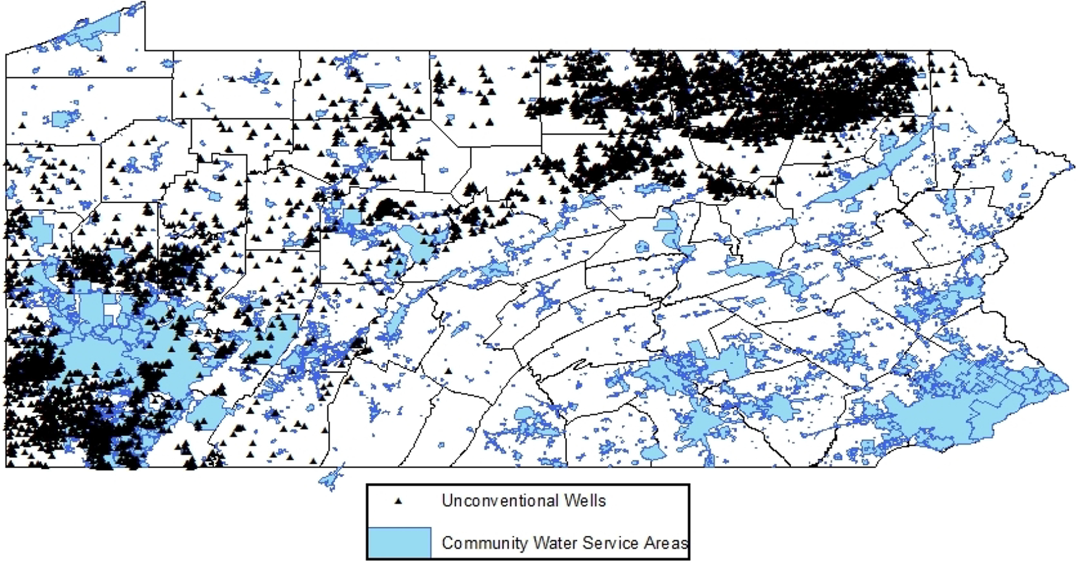
Gas Wells and Community Water Systems

With each birth spatially linked to every shale gas well within 10 kilometers of its water source (or residence), we then calculate the total number of wells within 10 kilometers of the infant’s CWS source (or residence) that were drilled within the gestation period of that infant. We use number of drilled wells as our measure of the intensive margin because the drilling process itself is most likely to impact ground water (as opposed to quantity of gas produced) and is also used in most other studies (Black et al., 2021; Bonetti et al., 2021).¹⁰ We additionally aggregate these “threats” at various buffers within 10 kilometers (i.e. between 1 and 5 kilometers) to distinguish the impact of threats at different proximities. We do this as there are typically multiple well bores (drilled at different times) located near any given groundwater source, and, as such, no clear “before” or “after” exposure period. While this complicates our definition of a treatment period, it provides good variation in exposure to shale gas operations that one can exploit. Figure 2, which delineates the new well bores drilled and the affected counties by year, is indicative of this as drilling varies both on the extensive and intensive margins. In these data, a quarter of gas wells are in production but are missing a drilling date. For the count of gas well threats in close proximity to water sources and residences, we impute the drilling date with the first production date minus 150 days, which is the average number of days between drilling and first production based on data from DrillingInfo, Inc. In Appendix Table 8.3.11, we verify that our results are robust to not imputing missing drilling dates and other forms of imputation.¹¹

Figure 2:

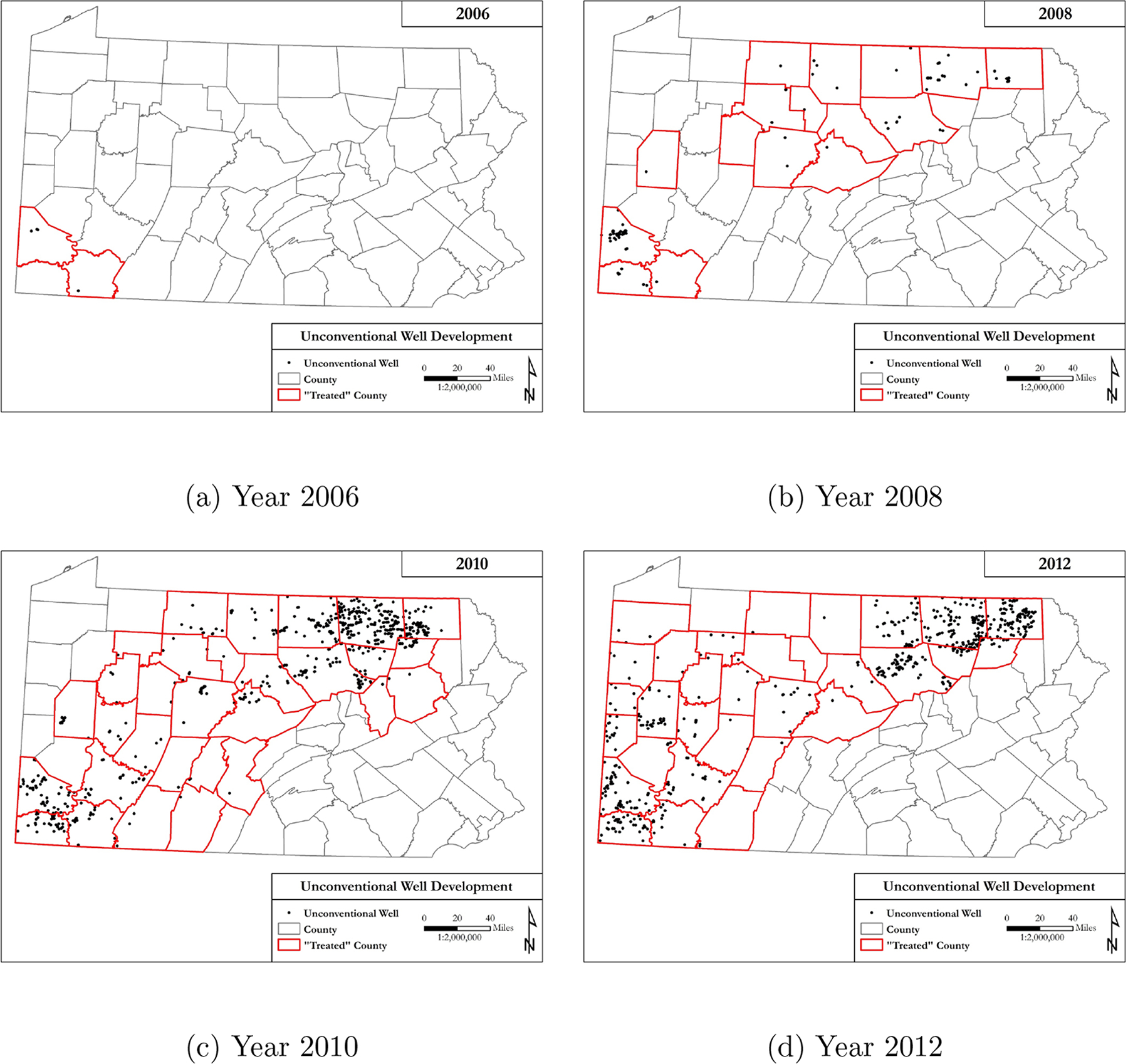
New Well Bores Drilled by Year

Our analysis sample is further restricted to residences that are within a community water system. The final estimation sample is thus composed of infants on ground water-sourced community water systems exposed to SGD within 10 km of their water source or residence. Table 1, Panel A presents the average exposure to drilled wells by water source and by residence. The average infant in our full sample is exposed during gestation to 0.002 shale gas wells within a kilometer of its source and 0.005 wells within a kilometer of its residence. Conditional on being exposed, the number of wells drilled respectively increases to 1.5 and 2.3. When we simply count the total (or cumulative) wells drilled before birth as opposed to focusing on within gestation, exposure through the source and the home respectively increases to 1.9 and 2.7, conditional on being exposed. Next, in anticipation of our fixed effects models, Table 1 Panel B counts the number of water systems and mothers that experience any change in exposure at the source. Of 49 systems with any water source within a kilometer of wells, infants in 42 systems experience some change in cumulative exposure to well bores versus those in 38 systems who experience changes in within-gestation exposure. Out of 1,541 mothers (within-mother sample Table 1 Panel B) who are exposed to gas wells within a kilometer of their source, 952 and 275 respectively experience a change in cumulative and gestational exposure (i.e., conceive children exposed to different amounts of gas wells).

Table 1:

Summary Statistics

	A. Average Exposure to Gas Wells by Infant (N = 325,439)
			Within Gestation		Cumulative
Proximity to Source		N	Mean	Mean | Exposed	Mean	Mean | Exposed
< 1km		8,142	0.002	1.525	0.011	1.944
< 3km		37,127	0.035	2.640	0.185	5.247
< 5km		83,011	0.103	3.886	0.566	7.899
< 10km		129,567	0.458	7.575	2.481	21.523
Proximity to Residence		N	Mean	Mean | Exposed	Mean	Mean | Exposed
< 1km		11,735	0.005	2.268	0.027	2.700
< 3km		81,203	0.088	3.412	0.474	6.326
< 5km		154,288	0.330	4.609	1.736	10.864
< 10km		303,463	1.685	7.723	1.685	4.588
Imputed		N	Mean	Mean | Exposed	Mean	Mean | Exposed
Source<1km		8,142	0.004	2.116	0.030	2.794
Residence<1km		11,735	0.006	2.226	0.038	2.914
	B. Count of Exposed Water Systems or Mothers
	Within CWS (N = 574)			Within Mom (N = 67,987)
Count:	Systems	Δ Cum. Exposure	Δ Gest. Exposure	Moms	Δ Cum. Exposure	Δ Gest. Exposure
Source<1km	49	42	38	1,541	952	275
Source<3km	205	173	155	7,500	3,783	1,825
Source<5km	270	244	230	16,937	9,917	4,210
Source<10km	420	357	340	26,714	10,332	6,616

Note. Table provides summary statistics of exposure to gas wells by births, water systems, or mothers. The final sample is composed of infants on ground water-sourced community water systems exposed to SGD either within 10 km of their water source or residence.

We use a similar procedure to construct our water quality data for water measurements beginning from 2011 through the third quarter of 2015, where a unit of observation is a contaminant sampling measurement (in parts per million or ppm) on a particular date.¹² For each water measurement, we aggregate the total number of well bores within 10 kilometers of the CWS source (and various proximities within) that have been drilled by the time that water measurement was taken. We remove samples that are greater than the 99th percentile of the sampling result distribution to prevent outliers from driving our results. Focusing on the set of contaminants that have been associated with SGD: of the 171,615 water measurement observations from systems within 10 kilometers of CWS sources, approximately 40% (or 69,239) are contaminants that have been tied to SGD. For this SGD-related sample, there are, respectively, 0.18, 0.45, and 27 well bores drilled, on average, within 1, 1.5 and 10 kilometers of source locations (Appendix Table 8.3.3).

3. Empirical Strategy

Birth Outcomes

Our baseline specification follows a difference-in-differences (DD) approach. We compare changes in birth outcomes (in response to drilling during gestation) for infants born in systems with drinking water sources near drilled wells to similar changes for infants in systems with sources that are farther away but still within 10 kilometers. Previous literature has found impacts on ground water quality using private wells from as close as 1 kilometer to as far as 5 (Johnston et al., 2018). To allow the data to inform us of the exposure buffer, we estimate the drilling impacts at 1-kilometer bins for distances to the source of between 0 and 5 kilometers. Specifically, we regress the birth outcome (Y_ijt) for a birth i in CWS j at time t on the number of well bores drilled during the infant’s gestation period at different distances from the CWS source:¹³

$$Y_{ijt}=\sum _{\ell =0}^4{\beta }_{\ell }{\mathit{\text{wells}}}_{ijt}^{(\ell ,\ell +1]}+{\beta }_5{\mathit{\text{wells}}}_{ijt}^{\le 10}+{\beta }_6{\mathit{\text{Rwells}}}_{ijt}^{\le 1}+X_{it}+m_t+cw{s}_j+{ϵ}_{ijt}$$ (1)

The main birth outcomes we examine include birth weight (grams) and gestation length (weeks), as well as indicators of low birth weight (weight < 2500 grams) or prematurity (gestation length < 37 weeks). The explanatory variables, ${\mathit{\text{wells}}}_{ijt}^{(\ell ,\ell +1]}$, gives the total number of well bores within (ℓ, ℓ + 1] kilometers of infant i’s water source that are drilled during gestation, for ℓ = 0, …, 4. The variable, ${\mathit{\text{wells}}}_{ijt}^{\le 10}$, returns the exposure to wells drilled during gestation within 10 kilometers of water sources, capturing air exposure from, for example, trucking activity. We also control for in utero exposure to the number of well bores drilled within 1 kilometer of the maternal residence during gestation, ${\mathit{\text{Rwells}}}_{ijt}^{\le 1}$, in all models, following previous work that has found proximity impacts on infant outcomes within this buffer (Hill, 2013; Currie et al., 2017). Our main coefficients of interest β₀ − β₄ returns the change in birth outcome given an increase in number of well bores within a specific buffer of the mother’s water sources, relative to the impact of drilling between 5 and 10 kilometers.

Causal inference based on the estimated relationship rests on the assumption that birth impacts captured by drilling activities that are “far” from water sources represent changes in infant health that would have occurred in the absence of drilling near the source. With the appropriate exposure buffer (discussed later in section 4 on results), we separate our infants into a treatment and control group to check for pre-existing trends in birth outcomes before SGD and find no evidence of differential trends in outcomes prior to 2009, when large-scale drilling began in PA.¹⁴ The main specification includes a number of additional control variables. Controls for maternal characteristics, X_it, include the mother’s age, race, education, enrollment in Medicaid and in the Special Supplemental Nutrition Program for Women, Infants, and Children (WIC) at birth, and a host of pregnancy risks (e.g. pre-gestational diabetes and smoking).¹⁵ We also include the following controls: average gestational temperature and precipitation near the maternal residence, which can directly impact birth outcomes (Deschênes et al., 2009) as well as vary exposure to water contaminants;¹⁶ a direct measure of changes in water quality of the mother’s water system that is not related to SGD, which is in the form of the number of coliform and disinfectant by-product exceedances of federally established legal limits during gestation;¹⁷ and the number of permitted well bores during an infant’s gestation – this can control for differences in expected well productivity, which can impact fertility and birth outcomes through local economic development (Kearney and Wilson, 2018; Hill, 2018).¹⁸ In addition, we include month-by-year fixed effects (m_t) and a fixed effect for each CWS, cws_j. These help to control for seasonal differences in birth outcomes and unobserved differences across water systems that might impact health. In certain specifications, we limit time-invariant, unobserved differences in family backgrounds with comparisons within siblings, i.e. through the use of mother fixed effects.¹⁹

We augment our baseline specification to ensure that the impacts we recover are through the mechanism of water contamination. Of utmost concern is that our estimated infant health impacts could be driven by changes in air quality (Chay and Greenstone, 2003; Currie and Neidell, 2005; Almond et al., 2009; Currie and Walker, 2011; Schlenker and Walker, 2016; Isen et al., 2017; Alexander and Schwandt, 2019). The negative impacts on health from other media of contamination that would most affect mothers living in close physical proximity to gas well activity would cause us to overstate the impacts of water quality changes. There are potential benefits, however, from living in close proximity of drilling activity if a household receives royalties or lease payments for allowing drilling on its property. Beyond the inclusion of gas well exposure via the maternal residence, we address air quality concerns more directly by including several controls to capture potential air quality impacts on birth outcomes. First, we control for a measure of ambient air quality at the Census block-group-by-year level that is calculated from TRI data using EPA’s Risk-Screening Environmental Indicators (RSEI) Model. Second, SGD-related transport is hypothesized to increase air pollutants; we control for the distance between maternal address and the closest PA state-owned and maintained public road to reduce the possibility that our results are caused by traffic-induced air quality changes.

Our empirical health model is grounded in the conceptual framework laid out in several important papers, notably Heckman (2007), Almond and Currie (2011), and Almond et al. (2018). Our problem of measuring the impact of SGD on health can be cast in a similar two-period health production model, modified to focus on the production of neonatal health based on parental investments in response to SGD. Under certain substitutability assumptions in health production, parental investments are compensatory. Thus, parents would increase investment in infant health to counter a negative shock such as SGD (Almond and Currie, 2011). The monetized health impact of SGD that ignores these behaviors would underestimate the true costs. On the other hand, the local impacts of SGD could be positive (e.g., from royalties) or negative (e.g., due to pollution) (Bartik et al., 2019; Muehlenbachs et al., 2015), meaning that even if responses are compensatory, whether investment actually increases depends on whether the net impacts of SGD are positive.

Our quasi-experimental framework is set up to both limit the parental response and identify a negative water pollution impact. The exposure definition based on water sources allows us to control for the wells drilled near residences, which helps to remove the local impacts from shale development due to mineral rights (positive) and local disamenities such as air pollution (negative). By doing so, we are more likely to isolate the negative, water-related portion of the SGD shock. Next, the exposure definition reduces the salience of SGD activities to households since people are unlikely to be aware of and respond to the threat at their water source,²⁰ which allows us to better control the mitigation response. With parental investments fixed (in response to shocks), then the impact that we measure is closer to an estimate of the pure biological impact of shocks on health (Royer, 2009).

Water Quality

Finally, whether SGD has impacted birth outcomes through drinking water quality requires understanding whether drinking water is actually impacted. Currently, there is no consensus regarding this “first stage” question from the scientific community. As such, establishing this relationship is an important, necessary step to asking the question of whether SGD impacts health through water; if no direct water quality impacts exist, then the scope for SGD impacts to be mediated through water would be indeed limited.

The model to estimate water quality impacts builds upon previous work in Hill and Ma (2017) and follows that for infant health closely. Our specification is again a difference-in-differences approach that compares water quality changes (in response to drilling) at water systems with sources near well bores to that for systems with sources between 5 and 10 kilometers. Specifically, we model the logarithm of water quality measurement i (ppm), r_ijt, for a community water system j to depend on the number of well bores drilled at different buffers within 10 kilometers.

The regression controls for sample-specific attributes (X_it) such as hour-of-day of when a sample was collected, the laboratory at which sampled results were measured, the contaminant group to which a pollutant belongs, sample type (distribution, entry point, etc.), number of MCL violations in the previous 30, 90 and 180 days, and temperature and precipitation. We also include county-by-year fixed effects (ν_jt), month-of-year fixed effects (m_t), and a fixed effect for each CWS, cws_j. The following gives our baseline specification:

$$r_{ijt}=\sum _{\ell =0}^4{\beta }_{\ell }{\mathit{\text{wells}}}_{ijt}^{(\ell ,\ell +1]}+{\beta }_5{\mathit{\text{wells}}}_{ijt}^{\le 10}+X_{it}+{\nu }_{jt}+m_t+cw{s}_j+{ϵ}_{it}$$ (2)

where ${\mathit{\text{wells}}}_{ijt}^{(\ell ,\ell +1]}$ denotes the number of well bores between ℓ and ℓ+1 kilometers of the water source drilled by time t. The parameters of interest, β_ℓ for ℓ = 0…4, return the impact of drilling an additional well bore between ℓ and ℓ + 1 kilometers from the water source on SGD-related contaminants, relative to changes in water quality trends over the same period as captured by water quality changes at water systems with more distant gas well threats. As with the infant health model, we check the validity of the parallel trends assumption and find no evidence that of pre-existing trends between water quality provided by systems near and far from drilling.²¹

We can explore the heterogeneity of effects by distinguishing the impacts from well bores that are drilled uphill versus downhill from sources, and those that ever produce any oil or gas as opposed to never-produce. In each case, the total number of threats within a certain proximity can be decomposed into those from each type of threat for a given way of distinguishing threats,

$${\mathit{\text{wells}}}_{ijt}^{(\ell ,\ell +1]}=\mathit{\text{Type}}{A}_{ijt}^{(\ell ,\ell +1]}+\mathit{\text{Type}}{B}_{ijt}^{(\ell ,\ell +1]}$$ (3)

where ‘TypeA’ and ‘TypeB’ would refer to, for example, the number of up- and down-gradient threats within the (ℓ, ℓ + 1]-kilometer interval when separately estimating impacts by elevation. Gas well threats are defined to be ‘uphill’ from a ground water source if the surface elevation of the well bore is higher than the surface elevation at the source intake. If elevation affects ground water flow, one would expect uphill threats to have stronger impacts on drinking water quality than those down hill of intake wells. Unproductive wells are typically left inactive because the cost is often prohibitive to permanently plug wells (Muehlenbachs, 2015). A priori, we do not know whether producing wells are more likely to contaminate nearby drinking water sources than wells that are just drilled and never produce. Separately testing these dimensions not only serves as robustness checks, but provides insight into potential mechanisms of contamination.

Our main analysis focuses on SGD-related chemicals; we estimate the impact of gas well threats on non-SGD related chemicals as a placebo check. We also test whether gas well threats that occur after water measurements are taken impact SGD-related chemicals. In addition, we assess the robustness of our water quality results with an additional data set on water sampling data from U.S. Geological Survey (USGS) ground water monitors. Construction of the data follows the same procedure as that used for public water system water quality, except the water sampling data is matched to gas wells via the location (i.e. longitude and latitude) of the USGS water monitor. The same specification is used as before, where controls for weather and contaminant group indicators are included, as well as fixed effects for month-of-year and county-year. These checks would further bolster the case that our estimated impacts are, in fact, causal.

4. Results

Water Quality

We first provide evidence that public drinking water quality has been compromised by shale gas development. Figure 3 plots the impacts on various water quality measures for both SGD and non-SGD chemicals.²² In Panel A of Table 2, we provide point estimates for a subset of these water quality measures, and additionally distinguish between gas wells drilled within 0.5 kilometers and 0.5 to 1 kilometers. In all regressions, we control for water system fixed effects, county-by-year fixed effects, and month-of-year fixed effects in addition to sample-specific characteristics.

Figure 3:

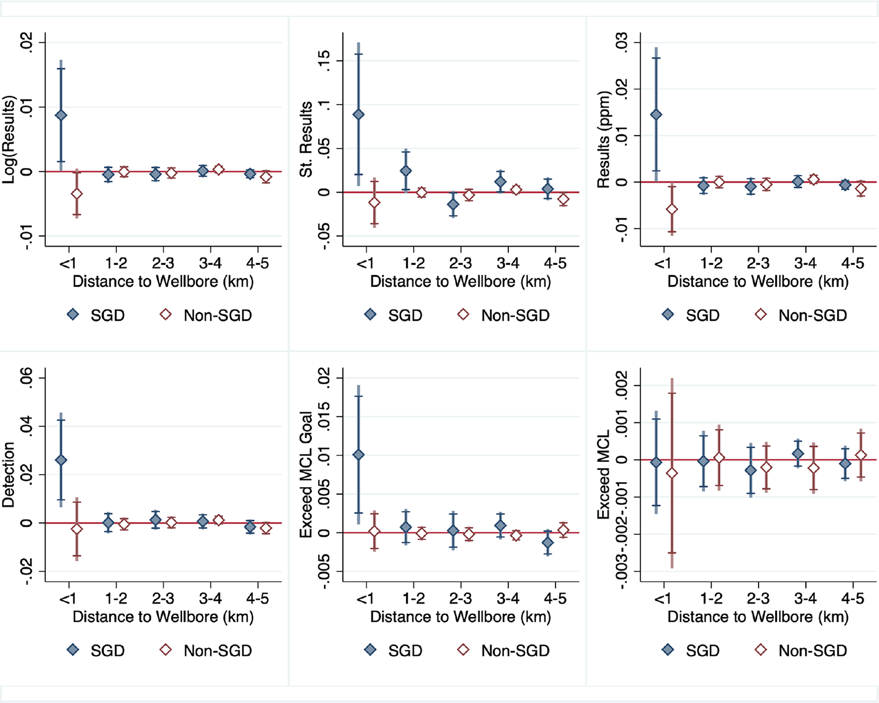
Water Quality Impacts

Note. Figure plots water quality impacts of drilling for SGD and non-SGD chemicals. The continuous measures are the sampling results in logs and levels (ppm), and ‘St. Result,’ which refers to sampling results that are standardized with respect to the mean and standard deviation of contaminants in its chemical group. The dichotomous measures include detection (results greater than 0), ‘MCL’ (the federally enforceable threshold for water quality), and ‘MCL goal,’ a more stringent public health goal for water quality.

Table 2:

Water Quality Impacts of SGD Chemicals

	A. Water Quality Impacts of Drilled Well Bores
Sample	SGD Chemicals			Non-SGD
Dep. Var.	Log Result	Detection	Std. Result	Log Result
Bores, <0.5km	0.0133** (0.00675)	0.0587*** (0.0166)	0.0840 (0.0716)	0.00245 (0.00417)
Bores, 0.5–1km	0.00907** (0.00413)	0.0263*** (0.00965)	0.0912** (0.0365)	−0.00280 (0.00230)
Bores, 1–2km	−0.000347 (0.000772)	2.26e-05 (0.00209)	0.0273** (0.0118)	0.000364 (0.000468)
Bores, 2–3km	−0.000300 (0.000618)	0.00146 (0.00197)	−0.0135* (0.00740)	−0.000255 (0.000449)
Bores, 3–4km	0.000148 (0.000528)	0.000737 (0.00164)	0.0103* (0.00618)	0.000324 (0.000337)
Bores, 4–5km	−0.000247 (0.000427)	−0.00250* (0.00149)	0.00408 (0.00585)	−0.000857 (0.000537)
Obs.	69,237	69,237	65,573	102,370
	B. Heterogeneity & Placebo Tests (SGD Chemicals)
Dep. Var.: Log Result Threat Type:	Uphill (A) vs. Downhill	Produced (A) vs. Never Produced	Future Drilling	Permitted Wells
Type A Bores, <1km	0.0101** (0.00448)	0.0131* (0.00730)
Type B Bores, <1km	0.00497 (0.00321)	0.00555 (0.00402)
Bores, Next 180 days, <1km			0.00587 (0.00393)
Permitted Bores, <1km				0.00642 (0.00499)
Obs.	69,237	69,237	69,237	69,237

Note. Table presents water quality impacts of SGD. Each column is a separate regression. The estimation sample consists of either SGD or non-SGD related water measurements from ground water-based community water systems with any water source within 10 km of any gas well. In panel A, the main regressors of interest are drilled well bores (at various distances to the water source). Across columns, we vary the sample (SGD or non-SGD related) and the dependent variable. Panel B re-estimates the specification in column 1 of panel A, except (1) it does not separate out well bores drilled within 0.5 and 1 kilometer, and (2) either distinguishes well bores within 1 kilometer as being Type A (uphill or producing) or Type B (downhill or never producing), or (3) adds additional variables for which we would expect no impact (future drilling or permitted well bores). Impacts at 1 kilometer for “Future Drilling” and “Permitted Wells” in panel B are not shown. Robust standard errors in parentheses are clustered at the CWS level.

^***p<0.01,

^**p<0.05,

^*p<0.1.

These results make clear that drilling an additional gas well within 1 kilometer of water sources increases chemicals related to SGD in public drinking water. For example, well bores drilled between 0.5 and 1 kilometer of water sources increases average sampling of contaminants by 0.94 percent (p<0.05) and detection of SGD chemicals by 2.6 percentage points (pp) (p<0.01) or close to 11 percent given a 0.24 baseline rate of detection. If these estimated impacts result from correlated environmental changes, then one would likely see increases in non-SGD related chemicals as well. We see no such effects for non-SGD chemicals in Figure 3.²³ The impacts of gas wells drilled within 0.5 kilometers are generally larger in magnitude, but are estimated with less precision. This pattern is intuitive as we would expect that systems with sources further away from gas wells are less likely to be affected by surface spills or activity that might impact ground water. Gas well threats at distances farther than 1 kilometer are an order of magnitude smaller and are not statistically significant, indicative of no effect. This is consistent with most of the scientific work to date investigating ground water impacts (Johnston et al., 2018). Estimates are robust to two-way clustering on both the spatial (CWS) and temporal (month-of-year) dimensions. We additionally explore the heterogeneity of effects in panel B of Table 2. Because elevation affects groundwater flow, we differentiate the water quality impacts of uphill well bores from those downhill. Unsurprisingly, we find that it is the uphill threats that are disproportionately affecting drinking water quality. We also find that the effect of an additional gas well drilled is driven primarily by producing wells as opposed to wells that never produce.

We perform a number of placebo checks. Panel B of Table 2 presents the impact of well bores drilled 180 days after water measurements are taken (column 3), and finds that there is no effect of threats incurred in the future on drinking water quality. This would be the case if our estimates are causal. Permitting of well bores similarly has no impact on water quality (column 4).

In additional robustness checks, we re-estimate our main water quality model using alternative water outcomes (Appendix Table 8.3.4, panel A) and subgroups of chemicals (Appendix Table 8.3.4, panel B). We find evidence of increased detection of chemical groups that are consistent with the scientific literature on SGD and water quality: detection of inorganic compounds generally increases by 18% relative to the mean (p<0.05) and detection of lead increases by 190% (p<0.05). There is also some evidence that synthetic organic compounds have increased (50%, p<0.1). On the other hand, detection of nitrates and nitrites seems to have decreased. We present these results as we think they are interesting, but caution strong takeaways given the rare occurrences of many of these chemicals (e.g. synthetics and nitrates/nitrites are both detected only 0.58 percent of the time in our sample).

The estimated effects on SGD chemicals in ambient water as captured by USGS water monitors are qualitatively similar (Appendix Table 8.3.5). In particular, the marginal impact of wells drilled within a kilometer of USGS ground water monitors is, on average, 3.0 percent (p<0.01). The estimated effect increases to 6.2 percent (p<0.01) for wells drilled upgradient to monitors, and 3.3 percent (p<0.01) for those that are ever in production. As before, the magnitude of impacts is smaller and not statistically significant for non-SGD related chemicals.

We highlight two additional findings that have policy implications. First, we find no evidence that the number of exceedances of the legally binding threshold for contaminants (i.e., the Maximum Contaminant Level (MCL)) has increased (Figure 3). However, we do find a 13% increase in samples that exceed public health goals (i.e., MCL goals). In other words, while the contaminant increases are not large enough to trigger MCL violations from the state water authority, they may still have measurable health impacts. This echoes work that finds the benefit-cost ratio of current US water regulations to be uncertain once a more comprehensive set of regulation benefits are included (Keiser et al., 2019). Second, the estimated impacts from water quality monitors are somewhat larger, suggesting that public water systems are at least partially successful at mitigating the impacts of water contaminants.

Our results clearly support the hypothesis that water quality has been compromised by shale gas operations. The magnitude of the contamination, however, is less clear. Several chemicals measured in the USGS water monitoring data are not present in the public drinking water data (e.g. bromides and chlorides) because they are not regulated under the Safe Drinking Water Act. In fact, 97.5 percent of SGD chemicals listed in the aforementioned EPA report are not sampled by public drinking water systems due to the same reason. Moreover, our estimated impacts examine the cumulative impact of drilling on water quality since we cannot assign “gestation periods” to water samples as we do for infants. These considerations indicate that the cumulative drinking water quality impacts based on measurements of regulated contaminants are likely understated. This has implications for the interpretation of our results and policy, a point we return to in later discussion.

Infant Health Impacts

We found robust evidence that public drinking water quality was compromised by shale gas development near water sources, which leads us to investigate the potential for health impacts. We present the average impacts of increasing the number of drilled wells on health outcomes in Table 3 with fixed effects for the public water system (panel A) and mother fixed effects (panel B).²⁴ In all regressions, we control for maternal characteristics, pregnancy risks, temperature and precipitation, number of disinfectant byproduct and coliform MCL violations, number of well bores drilled <1 km of the residence, and month-by-year fixed effects described in Section 3. Standard errors are clustered at the level of the fixed effect. The main estimates are plotted in Figure 4.

Table 3:

Within-Gestation Drilling Birth Impacts

A. Water System (CWS) Fixed Effects
Dep. Var.:	Gestation Length	Birth Weight	Premature	Low Birth Weight
Bores, <1km	−0.152*** (0.0395)	−24.92*** (8.593)	0.0104** (0.00485)	0.00850* (0.00449)
Obs. Mean	325,419 38.56	325,419 3292	325,419 0.0952	325,419 0.0772
B. Mother Fixed Effects
Dep. Var.:	Gestation Length	Birth Weight	Premature	Low Birth Weight
Bores, <1km	−0.157*** (0.0502)	−26.10* (13.78)	0.0152** (0.00750)	0.0123* (0.00720)
Obs. Mean	152,944 38.40	152,944 3267	152,944 0.114	152,944 0.0924

Note. Table presents estimated impacts of bores drilled within 1 kilometer of CWS sources on birth outcomes relative to well bores drilled between 5 and 10 kilometers. Each column represents a separate regression, where the mean of the dependent variable is provided in the last row. The impacts of drilling in areas between 1 and 5 kilometers from the source are included in the regressions, but not shown. All regressions control for maternal characteristics, pregnancy risks, temperature and precipitation, # of coliform and disinfectant by-product MCL violations, # of bores drilled <1km of the residence, and fixed effects for the month-of-year and for the water system. Panel B includes fixed effects for the mother. The estimation sample is composed of infants on ground water-sourced community water systems exposed to SGD either within 10 km of their water source or residence. Standard errors are clustered at the level of the fixed effect.

Figure 4:

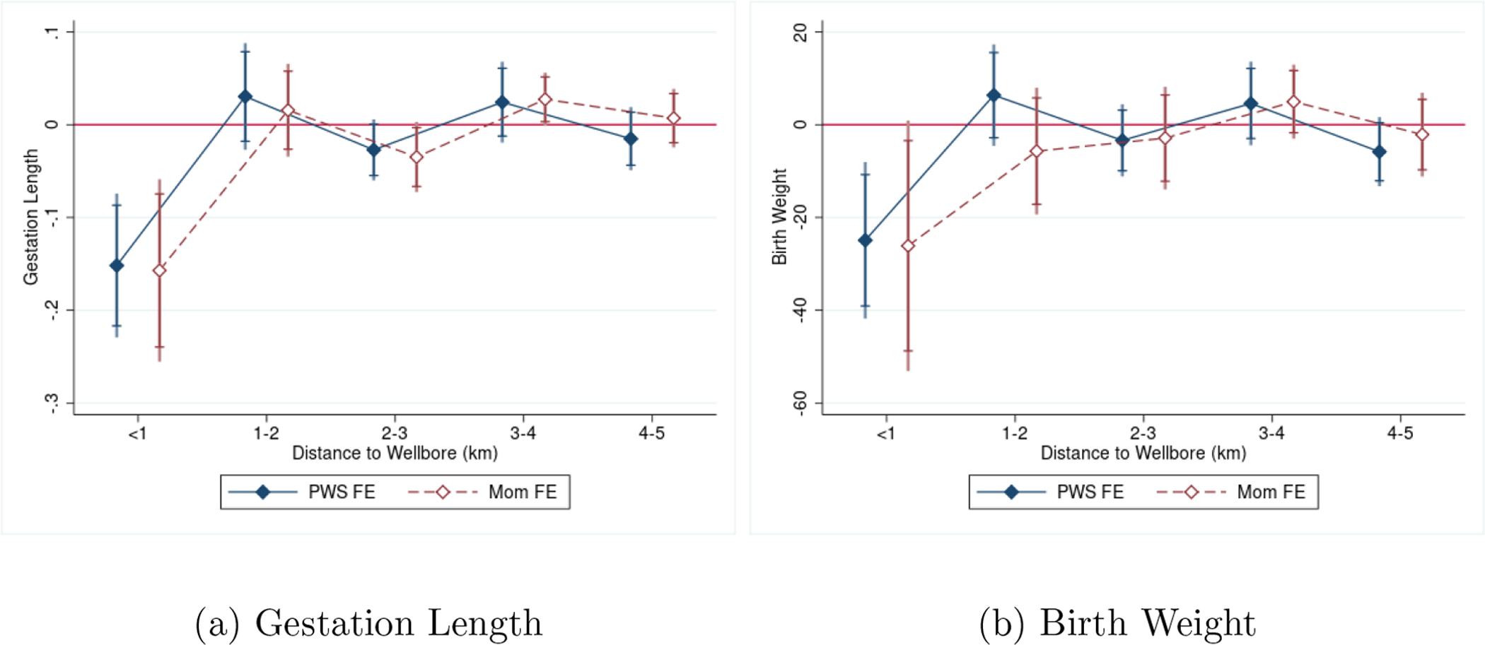
Birth Impacts of Drilling within Gestation

Estimation of the CWS and mother fixed effects (FE) models find fairly precise impacts of drilling within 1 kilometer on gestation length — each gas well drilled within 1 kilometer of an infant’s water source during pregnancy reduces gestation length by between 0.13 weeks (Mom FE, p<0.05) to 0.15 weeks (CWS FE, p<0.01). In terms of birth weight, each well bore decreases birth weight by 24.9 grams (p<0.01) when controlling for CWS fixed effects and by 26.1 grams with the inclusion of mother fixed effects (p<0.1).²⁵ Researchers commonly use binary metrics of whether births are preterm, meaning that the fetus had a gestation length of less than 37 weeks, and whether birth weight is at least 2500 grams, below which is considered a low birth weight infant. These thresholds denote levels at which medical interventions are often necessary, and provide outcomes that are easier to assign economic costs to in a cost-benefit assessment. We examine these threshold outcomes in the last two columns of Table 3. Impacts on the incidence of prematurity range from 1.0 pp and 1.5 pp (p<0.05). Given an average incidence of prematurity of 9.5 percent for the CWS FE sample and 11 percent for the Mom FE sample, these effects translate to about an 11–13 percent increase in chance of preterm birth. The increased incidence of low birth weight is respectively 0.85 and 1.2 pp for the CWS and mother fixed effects models (p<0.10), which also translate to an effect of around 11 to 13 percent.²⁶ Our main estimates with CWS fixed effects are robust to two-way clustering on CWS and birth month-of-year.

To contextualize the magnitude of our findings, Grossman and Slusky (2019) find an 8-gram reduction in average birth weight (BW) for the crisis in Flint, Michigan and Flynn and Marcus (2021) find Clean Water Act grants increased BW by 8-grams. For low birth weight (LBW) and preterm birth (PTB), Marcus (2021) find exposure to a leaking underground storage tank during gestation increases the probability of LBW and PTB by 7–8 percent, Dave and Yang (2020) find increased lead in Newark, NJ drinking water increased LBW and PTB by 14–22 percent, and DiSalvo and Hill (2019) find increases in LBW and PTB of 6 and 10.2 percent, respectively, in response to large increases in water contamination below regulatory limits. Related literature on residential proximity to SGD and infant health also finds an ~25 percent increase in chance of LBW (Currie et al., 2017; Hill, 2018). Considering the quantified impacts of neonatal health on future outcomes discussed earlier, the magnitudes of our estimated effects are meaningful.

5. Robustness and Heterogeneity of Effects

This section evaluates the robustness of our estimated impacts with placebo tests and heterogeneity analysis. We assess whether impacts are driven by compositional changes reflecting the types of mothers who choose to have children or migration/sorting. We also evaluate the extent to which our estimates are driven by correlated changes in environmental nuisances in areas with drilling. We explore heterogeneity of impacts based maternal characteristics and the timing of drilling impacts. Additional robustness checks are presented in the appendix, including the effect of limiting to singleton births, alternative imputations for missing drilling dates, and reverse causality.

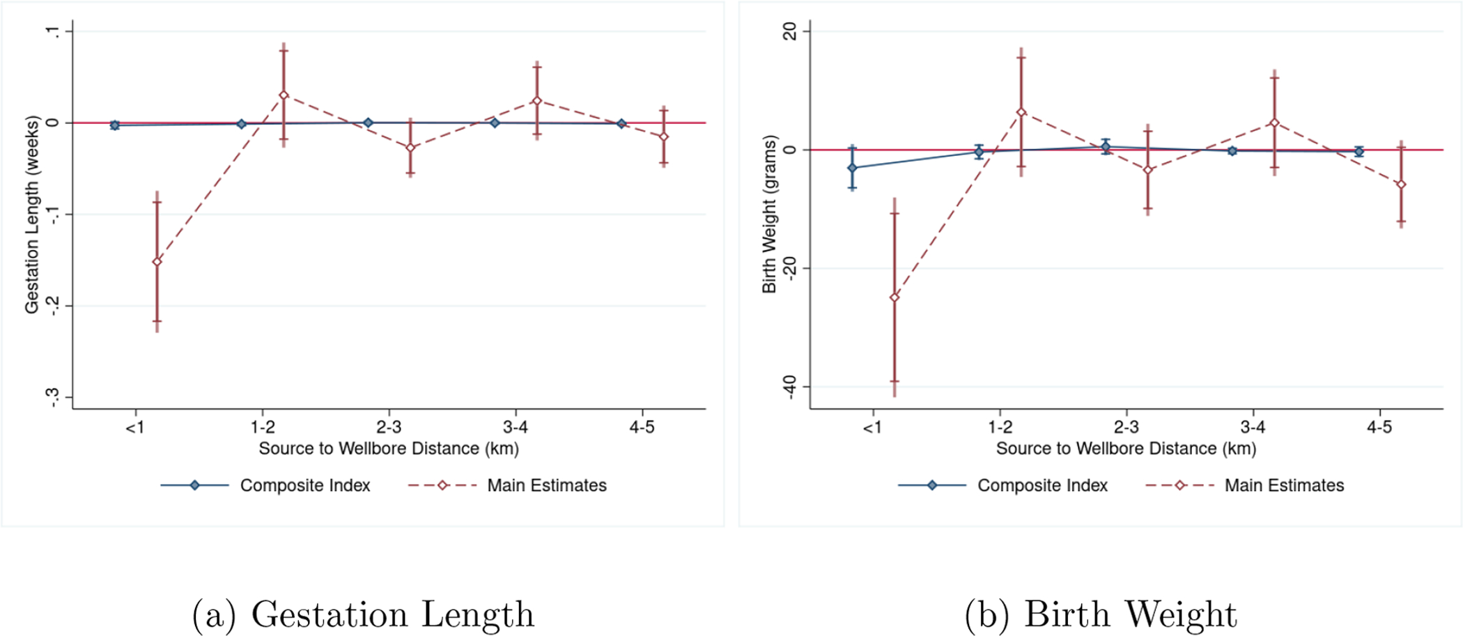
Various behavioral responses are important to consider when interpreting our results. In response to environmental risks, exposed groups may switch to bottled water (Graff Zivin et al., 2011; Wrenn et al., 2016), alter fertility decisions (Kearney and Wilson, 2018), or move (Banzhaf and Walsh, 2008). If mothers engage in such avoidance measures, then our estimates might be driven by changes in sample composition in response to gas well development. We first test whether our results reflect compositional changes in the types of mothers who select into fertility near gas well development. We create a composite index of selection factors by projecting birth outcomes on to maternal characteristics, and then use the predicted outcomes as the dependent variable in our main specifications of interest. If our estimates are not driven by selection, then we should not see evidence that drilling yields an effect in these projected outcomes. We plot the resulting coefficients on drilling at different distances to water sources in Figure 5 along with our main effects for comparison. We do not find evidence that our effects are driven by maternal composition.

Figure 5:

Impact of Drilling on Composite Index of Mother Characteristics

Note. Figure plots the impact of drilling on a projection of birth outcomes on maternal characteristics and compares it to our main estimates of the birth impact. Specifically, we regress birth outcomes onto maternal characteristics, predict the outcomes based on thes characteristics, and then use the predicted outcomes as the dependent variable in our main specifications of interest.

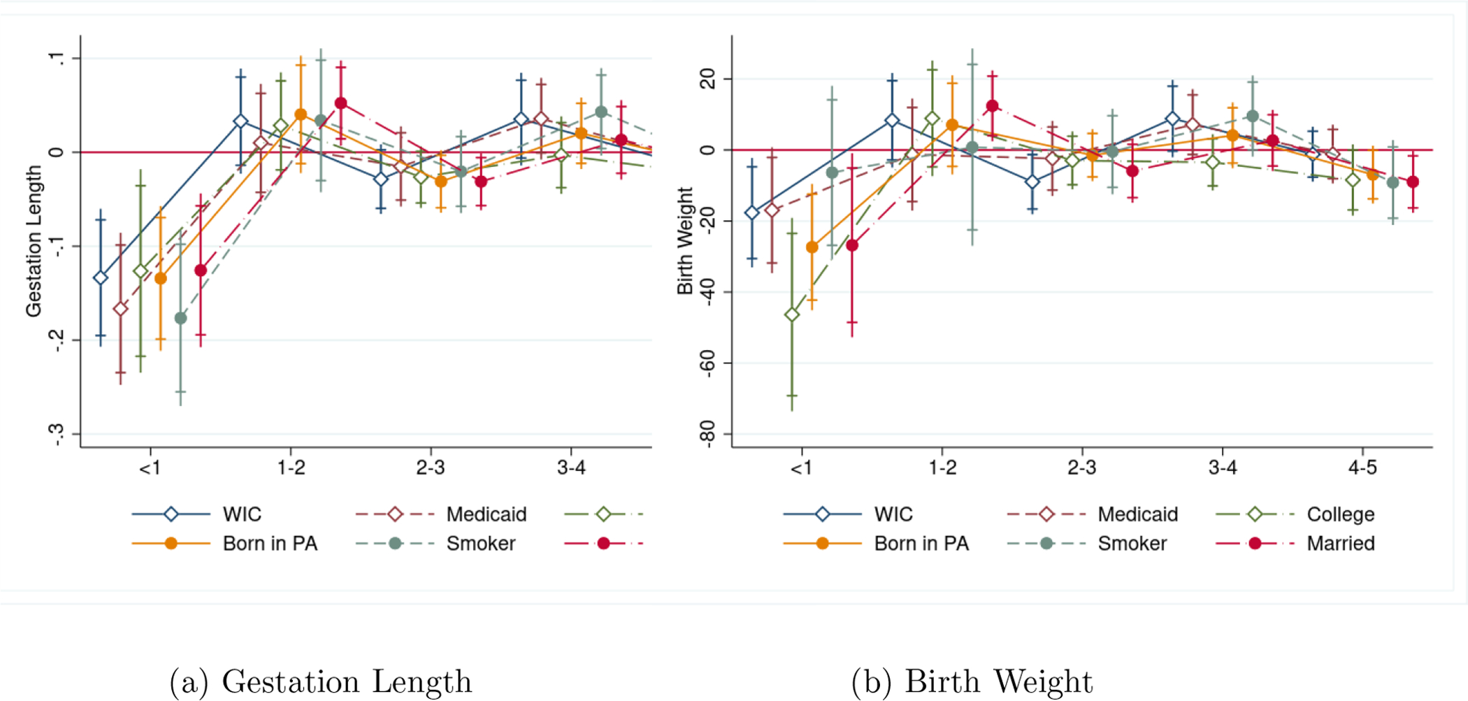
We also estimate our birth impacts using subgroups based on the mother’s socioeconomic status (SES), such as educational attainment and Medicaid use. If individuals are indeed taking measures to mitigate exposure, then the largest negative health impacts should be concentrated among the low SES groups, those with arguably less ability to invest in costly avoidance measures (Neidell, 2009; Currie et al., 2013). Figure 6 plots the impacts (using CWS FE) against exposure distance by SES sub-group. There is no evidence that infants born to more economically disadvantaged mothers are disproportionately affected. If anything, we actually find that college-educated women see somewhat larger impacts. If educational attainment is also an indicator of income, then this would suggest avoidance behavior is less likely to be an issue.

Figure 6:

Impacts by Mother’s Socioeconomic Status

Next, we test for a sorting response using the sample of mothers for whom we observe multiple births. Table 4 estimates whether mothers are more likely to switch water systems or ZIP codes in response to an additional gas well drilled within the vicinity of their water source (columns 1 and 2) or near their residence (columns 3 and 4). The same set of controls used in the specifications of Table 3 are used, and CWS fixed effects are included for all specifications. We find no statistically significant impacts of gas well activity near water sources on the likelihood to move. Interestingly, we do find some evidence that well bores drilled in close proximity of the maternal residence increases the chance of moving. That mothers are not so responsive to drilling in our setting is potentially reasonable if SGD near water sources are less observable than that near the residence: the two types of exposure are highly, but not perfectly, correlated, and mothers may assume that piped public water protects them from contamination from the industry, as indicated by perceived risks being primarily associated with private ground water wells (Muehlenbachs et al., 2015). We test that our results are similar when we remove mothers whose residence is within 1 km of any gas well to ensure that selective migration in response to drilling near the residence is not driving our results.²⁷ These findings bolster our identification strategy using water source locations to define exposure. We infer from these tests that our estimated impacts of SGD on birth outcomes are not driven by differential sorting or fertility decisions by maternal SES in response to gas well development.

Table 4:

Probability of Moving

Drilling Location:	Near Water Source		Near Residence
Dep. Var.:	Switch CWS	Switch ZIP	Switch CWS	Switch ZIP
Bores, <1km	−0.00373 (0.0121)	−0.00166 (0.00957)	0.0202*** (0.00763)	0.0149*** (0.00529)
Bores, 1–2km	−0.00686 (0.00569)	−0.00741 (0.00547)	−3.39e-05 (0.00298)	0.000189 (0.00259)
Bores, 2–3km	0.00206 (0.00414)	0.00148 (0.00450)	−0.000984 (0.00277)	0.00396* (0.00238)
Bores, 3–4km	−0.00147 (0.00236)	−0.000625 (0.00286)	0.000247 (0.00204)	0.000950 (0.00143)
Bores, 4–5km	0.000384 (0.00247)	−0.00164 (0.00312)	−0.00173 (0.00174)	−0.00197 (0.00179)
Obs.	152,944	152,944	142,773	142,773
Mean	0.308	0.409	0.314	0.403

Note. Table regresses an indicator for whether a mother switched water systems or ZIP codes on the number of gas wells drilled within the vicinity of a CWS source (“Near Water Source”) and the maternal address (“Near Residence”) using the sample of mothers who we observe to have multiple births. The same set of controls as the specifications of Table 3 are used (see Table 3 for a description). Dependent variable means are provided in the last row. For all specifications, CWS fixed effects are included.

As Pennsylvania has had a history of coal mining dating back to the 1920’s, one may be concerned that our estimates are picking up the impact of these activities, which often coincide with areas that are currently engaged in SGD.²⁸ To this end, we identify the public water systems that have any drinking water sources within 1, 5 and 10 km of historical coal seams or any coal seams (active or historical), and estimate our model on a sub-sample that removes infants who belong to any of those groups. Doing so reduces the potential for coal mining to explain our estimates. Results are stable regardless of how we limit the distance between coal seams and water sources (Appendix Table 8.3.9).²⁹

In our analysis of the timing of drilling and water quality, we find that SGD-related contamination increases 90 days after the drilling of the well (spud date). The contamination continues for up to 270 days after drilling and then returns to baseline. With this in mind, we estimate the health impacts of the cumulative number of gas wells drilled before birth. As expected from our analysis on timing, the magnitudes of the impacts decrease, suggesting that it is in utero threats that matter the most.³⁰ Our current data on SGD stages, however, is limited (e.g. we do not observe the timing of fracking). We are therefore unable to identify the exact SGD processes (e.g., drilling, spills, hydraulic fracturing, production, casing failures, tank leaks) that are causing the health effects that we find. Our analysis, however, suggests that most of the impacts are concentrated in the period immediately after drilling. Future work should explore the specific weaknesses of the process causing groundwater contamination.

We perform additional robustness checks available in the Appendix. Well bores drilled after an infant is born do not impact birth outcomes (Appendix Table 8.3.10), and the impacts on singleton births are similar. In Appendix Table 8.3.11, we show how various forms of drilling date imputation changes our results. The absence of imputation increases the magnitude of our results and other forms of imputation do not change the qualitative conclusions. Together, these results lead us to believe that unconventional drilling has had an independent impact on birth outcomes through contamination of public drinking water.

6. Discussion

We set out to examine the infant health impacts of water pollution using exogenous variation in water quality caused by shale gas development near drinking water sources. Our findings indicate that drilling near an infant’s public water source yields poorer birth outcomes and more SGD-related contaminants in public drinking water. We discuss the implications of our results for shale gas regulation and drinking water policy as well as their limitations.

Shale gas development creates multiple “first stage” effects on environmental quality: light, noise, air, and water pollution (Hill, 2018; Hill and Ma, 2017; McCawley, 2017; Casey et al., 2018; Zhang et al., 2019; Boslett et al., 2021; Black et al., 2021; Bonetti et al., 2021). It is important for policy to reconcile the shale gas and infant health literature and compare residential proximity health effects (Currie et al., 2017; Hill, 2018) to those measured in this paper from public water system source proximity. Table 5 begins by replicating the previous literature on the proximity impacts of SGD in column 1 using a binary indicator for having any well within 1 kilometer of the maternal residence prior to birth. Each subsequent column progressively alters the sample (column 2 and 3) or control variables (column 4) to be consistent with our main specification. The final column, which includes both source and residential proximity exposures to SGD, finds that each additional well drilled during gestation within 1 km of a public water source increases the risk of low birth weight by about 0.71 pp and any well drilled within 1 km of the residence increases low birth weight by 0.68 pp.³¹

Table 5:

Comparison of Well Bore Threats near Home versus Source

Dep. Var.: Low Birth Weight Model:	Previous Literature	Full Sample: Near Home or Source	Sample Limit: Public Water	Add Controls	Add Water Source Threats
Any Well <1 km of Home	0.00745* (0.00385)	0.00876*** (0.00303)	0.0124*** (0.00425)	0.00661 (0.00401)	0.00678* (0.00401)
Wells <1 km of Source					0.00707* (0.00402)
Observations	290,732	398,724	321,691	325,419	325,419

Note. Table compares our estimated impacts for low birth weight along various dimensions of SGD exposure. As in Table 3, missing spud dates are imputed for all specifications. Column 1 follows previous literature and uses a binary indicator for having any gas well within 1 kilometer of the maternal residence prior to birth (2004–2013 years; residences within 10 km of shale gas wells). Column 2 expands to our full sample of 2003–2015 birth data and includes residences that are served by water systems within 10 kilometers of a shale gas well. Column 3 limits to only those residences served by public water. Column 4 includes our main specification controls (adding maternal, weather, and permit controls) and expands the sample to include residences either served by public water or located within 10 km of any gas well. Column 5 additionally controls for our main threat variable of interest, the number of gas wells drilled during gestation.

These results, combined with the current epidemiological and economic literature, are supporting the following conclusions. Shale gas development influences the environment by reducing ambient air quality and increasing ground water contamination. The effects for air quality (residential proximity) persist for multiple years after drilling and potentially at larger distances from the residence (Hill, 2018; Currie et al., 2017).³² The separate effects of water pollution from drilling at source locations are sustained primarily during gestation (i.e., these effects are more short term and less persistent). A policy to directly limit the health impacts from water pollution is to require a minimum “setback” distance at which drilling operations can take place near water sources. As minor reductions in surface area for extraction does little to obstruct access to subsurface resources with the innovations in horizontal drilling, modest setback requirements are likely to yield significant increases in benefits without the accompanying increase in economic costs.

With respect to the benefits of water quality control, we believe our results provide compelling evidence that water pollution causes negative infant health effects even at mild levels (i.e. at levels that do not trigger regulatory violations). The magnitudes of our infant health effects support water pollution as a potentially important contributor to various health and socioeconomic disparities in adulthood. The implied elasticity of health impacts with respect to regulated water contaminants in this paper, however, is likely to be an upper bound since we only observed SGD contaminants that are currently monitored under the Safe Drinking Water Act. The same issue also limits our ability to directly apply these results to re-assess drinking water policy.

Co-pollutants that are unobserved (either because the scientific community does not know of their existence or because sampling is not required) imply that our estimate of the SGD impacts on drinking water are understated. It also implies that the associated health impacts may be either due to an increase in observed, regulated contaminants or a correlated increase in unregulated contaminants that we do not observe. Since monetizing health impacts for benefit-cost analysis requires information on the effects of specific contaminants, our results are thus unable to speak to whether regulation should increase the stringency of existing contaminants or expand the set of regulated contaminants. Future work to collect and assess the health impacts of a more comprehensive set of water chemicals would be fruitful. It would be very expensive, however, for drinking water systems to regulate each of the 2500 suspected SGD contaminants. Our study supports a simple policy solution to confront the potentially massive number of SGD chemicals in water: mitigate water contamination at the source to prevent adverse infant health effects mediated through water pollution.

7. Conclusion

This study seeks to understand and quantify the impacts of drinking water quality on infant health while exploiting exogenous changes in water quality induced by shale gas development (SGD). Our novel data links together the locations of new mothers’ residences, community water system’s water source locations, and the locations of shale gas wells in Pennsylvania. We find robust and consistent evidence of an effect of shale gas development within 1 km of ground water sources on water quality. Importantly, we also find consistent evidence that water quality changes due to SGD produces measurable impacts on birth outcomes: the incidences of preterm birth and low birth weight increase by between 9 and 13 percent, respectively. We determine that our results are unlikely to be driven by correlated air quality changes associated with congestion/traffic or coal, nor are they driven by maternal mobility and fertility decisions in response to SGD. Our infant health impacts are similar in magnitude to air pollution studies, such as EZ-Pass reducing LBW and PTB by ~10% (Currie and Walker, 2011) or living downwind of coal plant increasing LBW by 6.5% (Yang et al., 2017).

Over three decades have passed since the enactment of federal regulations to protect our water resources. Despite successfully reducing water contamination in public drinking water systems, 9 to 45 million people, representing 4 to 28% of the US population, were affected by health-based violations between 1982 and 2015 (Allaire et al., 2018). Concurrently, SGD has been taking place near a non-trivial portion of the US population and has real potential to threaten water resources and health: 17.6 million people live within a mile of an oil or gas well (Czolowski et al., 2017) and 8.6 million people are served by water systems with sources within a mile of a well (U.S. EPA, 2016).

The paper’s findings indicate large social costs of water pollution through health and highlight drinking water as a specific exposure pathway for an emerging industry with little environmental regulation. In particular, our estimates reveal that SGD increases regulated contaminants found in drinking water, but not enough to trigger regulatory violations, and that these operations yield measurable health impacts that could either be due to increases in regulated water contaminants below the threshold or unregulated water contaminants that we, unfortunately, cannot observe. Future work to identify the sources of water contamination is needed to determine whether net benefits would arise from increasing the stringency of currently-regulated contaminants or expanding the set of regulated contaminants. Nonetheless, these findings suggest that the external costs of our water and resulting birth impacts are non-trivial. Researchers have shown that neonatal health has a significant effect on both mortality within one year and mortality up to age 17 (Oreopoulos et al., 2008). Further, these outcomes are strong predictors of a host of longer term outcomes, such as human capital accumulation, welfare take-up, earnings, and labor force participation (Black et al., 2007; Oreopoulos et al., 2008; Johnson and Schoeni, 2011; Figlio et al., 2014). Motivated by water pollution’s effects on infant health and the potential impacts on long-run measures of well-being, our work provides an impetus for the re-evaluation of existing drinking water policies and possibly the regulation of the shale gas industry.

References

- Aizer Anna, Currie Janet, Simon Peter, and Vivier Patrick. 2018. “Do Low Levels of Blood Lead Reduce Children’s Ruture Test Scores?” American Economic Journal: Applied Economics, 10(1): 307–41. [DOI] [PMC free article] [PubMed] [Google Scholar]
- Alexander Diane, and Schwandt Hannes. 2019. “The Impact of Car Pollution on Infant and Child Health: Evidence from Emissions Cheating.” IZA Discussion Paper No. 12427. [Google Scholar]
- Allaire Maura, Wu Haowei, and Lall Upmanu. 2018. “National Trends in Drinking Water Quality Violations.” Proceedings of the National Academy of Sciences, 115(9): 2078–2083. [DOI] [PMC free article] [PubMed] [Google Scholar]
- Allcott Hunt, and Keniston Daniel. 2017. “Dutch Disease or Agglomeration? The Local Economic Effects of Natural Resource Booms in Modern America.” Review of Economic Studies, 85(2): 695–731. [Google Scholar]
- Almond D, and Currie J. 2011. “Human Capital Development before Age Five.” Handbook of Labor Economics, 4(Part B): 1315–1486. [Google Scholar]
- Almond Douglas, Currie Janet, and Duque Valentina. 2018. “Childhood Circum-stances and Adult Outcomes: Act II.” Journal of Economic Literature, 56(4): 1360–1446. [Google Scholar]
- Almond Douglas, Edlund Lena, and Palme Mårten. 2009. “Chernobyl’s Subclinical Legacy: Prenatal Exposure to Radioactive Fallout and School Outcomes in Sweden.” Quarterly Journal of Economics, 124(4): 1729–1772. [Google Scholar]
- Anderson D Mark, Charles Kerwin Kofi, and Rees Daniel I. 2020. “Re-examining the contribution of public health efforts to the decline in urban mortality.” American Economic Journal: Applied Economics 143–75. [Google Scholar]
- Banzhaf Spencer H, and Walsh Randall P. 2008. “Do People Vote with their Feet? An Empirical Test of Tiebout’s Mechanism.” American Economic Review, 98(3): 843–863. [Google Scholar]
- Bartik Alexander W, Currie Janet, Greenstone Michael, and Knittel Christopher R. 2019. “The Local Economic and Welfare Consequences of Hydraulic Fracturing.” American Economic Journal: Applied Economics, 11(4): 105–55. [Google Scholar]
- Beach Brian, Ferrie Joseph, Saavedra Martin, and Troesken Werner. 2016. “Typhoid fever, water quality, and human capital formation.” The Journal of Economic History, 76(1): 41–75. [Google Scholar]
- Bennear Lori S., Jessoe Katrina K., and Olmstead Sheila M.. 2009. “Sampling Out: Regulatory Avoidance and the Total Coliform Rule.” Environmental Science & Technology, 43(14): 5176–5182. [DOI] [PubMed] [Google Scholar]
- Black Katie Jo, Boslett Andrew J, Hill Elaine L, Ma Lala, and McCoy Shawn J. 2021. “Economic, Environmental, and Health Impacts of the Fracking Boom.” Annual Review of Resource Economics, 13. [Google Scholar]
- Black Sandra E., Devereux Paul J., and Salvanes Kjell G.. 2007. “From the Cradle to the Labor Market? The Effect of Birth Weight on Adult Outcomes.” Quarterly Journal of Economics, 122(1): 409–439. [Google Scholar]
- Bonetti Pietro, Leuz Christian, and Michelon Giovanna. 2021. “Large-sample evidence on the impact of unconventional oil and gas development on surface waters.” Science, 373(6557): 896–902. [DOI] [PubMed] [Google Scholar]
- Boslett Andrew, Hill Elaine, Ma Lala, and Zhang Lujia. 2021. “Rural light pollution from shale gas development and associated sleep and subjective well-being.” Resource and Energy Economics, 64, p. 101220. [DOI] [PMC free article] [PubMed] [Google Scholar]
- Brainerd Elizabeth, and Menon Nidhiya. 2014. “Seasonal effects of water quality: The hidden costs of the Green Revolution to infant and child health in India.” Journal of Development Economics, 107 49–64. [Google Scholar]
- Casey Joan A, Wilcox Holly C, Hirsch Annemarie G, Pollak Jonathan, and Schwartz Brian S. 2018. “Associations of Unconventional Natural Gas Development with Depression Symptoms and Disordered Sleep in Pennsylvania.” Scientific reports, 8(1):, p. 11375. [DOI] [PMC free article] [PubMed] [Google Scholar]
- Chay KY, and Greenstone M. 2003. “The Impact of Air Pollution on Infant Mortality: Evidence from Geographic Variation in Pollution Shocks Induced by a Recession.” Quarterly Journal of Economics, 118(3): 1121–1167. [Google Scholar]
- Chetty Raj, and Hendren Nathaniel. 2018. “The Impacts of Neighborhoods on Inter-generational Mobility I: Childhood Exposure Effects.” Quarterly Journal of Economics, 133(3): 1107–1162. [Google Scholar]
- Cunha Flavio, and Heckman James. 2007. “The Technology of Skill Formation.” American Economic Review, 97(2): 31–47. [Google Scholar]
- Currie J, and Neidell M. 2005. “Air Pollution and Infant Health: What Can We Learn from California’s Recent Experience?” Quaterly Journal of Economics, 120(3): 1003–1030. [Google Scholar]
- Currie J, and Walker R. 2011. “Traffic Congestion and Infant Health: Evidence from E-ZPass.” American Economic Journal: Applied Economics, 3(1): 65–90. [Google Scholar]
- Currie Janet, Zivin Joshua Graff, Meckel Katherine, Neidell Matthew, and Schlenker Wolfram. 2013. “Something in the Water: Contaminated Drinking Water and Infant Health.” Canadian Journal of Economics, 46(3): 791–810. [DOI] [PMC free article] [PubMed] [Google Scholar]
- Currie Janet, Greenstone Michael, and Meckel Katherine. 2017. “Hydraulic Fracturing and Infant Health: New Evidence from Pennsylvania.” Science Advances, 3(12):, p. e1603021. [DOI] [PMC free article] [PubMed] [Google Scholar]
- Cutler David, and Miller Grant. 2005. “The Role of Public Health Improvements in Health Advances: The Twentieth-Century United States.” Demography, 42(1): 1–22. [DOI] [PubMed] [Google Scholar]
- Czolowski Eliza D, Santoro Renee L, Srebotnjak Tanja, and Shonkoff Seth BC. 2017. “Toward Consistent Methodology to Quantify pPopulations in Proximity to Oil and Gas Development: A National Spatial Analysis and Review.” Environmental Health Perspectives, 125(8):, p. 086004. [DOI] [PMC free article] [PubMed] [Google Scholar]
- Darrah Thomas H, Vengosh Avner, Jackson Robert B, Warner Nathaniel R, and Poreda Robert J. 2014. “Noble Gases Identify the Mechanisms of Fugitive Gas Contamination in Drinking-water Wells Overlying the Marcellus and Barnett Shales.” Proceedings of the National Academy of Sciences, 111(39): 14076–14081. [DOI] [PMC free article] [PubMed] [Google Scholar]
- Dave Dhaval M, and Yang Muzhe. 2020. “Lead in Drinking Water and Birth Outcomes: A Tale of Two Water Treatment Plants.”Technical report, National Bureau of Economic Research. [DOI] [PubMed] [Google Scholar]
- Deryugina Tatyana, Heutel Garth, Miller Nolan H, Molitor David, and Reif Julian. 2019. “The Mortality and Medical Costs of Air Pollution: Evidence from Changes in Wind Direction.” American Economic Review, 109(12): 4178–4219. [DOI] [PMC free article] [PubMed] [Google Scholar]
- Deschênes Olivier, Greenstone Michael, and Guryan Jonathan. 2009. “Climate Change and Birth Weight.” American Economic Review, 99(2): 211–217. [DOI] [PubMed] [Google Scholar]
- Deziel Nicole C, Brokovich Eran, Grotto Itamar, Clark Cassandra J, Barnett-Itzhaki Zohar, Broday David, and Agay-Shay Keren. 2020. “Unconventional Oil and Gas Development and Health Outcomes: A Scoping Review of the Epidemiological Research.” Environmental Research, p. 109124. [DOI] [PubMed] [Google Scholar]
- DiSalvo Richard, and Hill Elaine. 2019. “The Effects of Drinking Water Contamination on Birth Outcomes: New Estimates from Drinking Water Samples.” Working Paper. [Google Scholar]
- Ebenstein Avraham. 2010. “The Consequences of Industrialization: Evidence from Water Pollution and Digestive Cancers in China.” The Review of Economics and Statistics, 94(1): 186–201. [Google Scholar]
- EPA, US. 2015. “Information about Public Water Systems.” https://www.epa.gov/dwreginfo/information-about-public-water-systems, Accessed: 2021-11-16.
- Ferrie Joseph P, Rolf Karen, and Troesken Werner. 2012. “Cognitive Disparities, Lead Plumbing, and Water Chemistry: Prior Exposure to Water-Borne Lead and Intelligence Test Scores among World War Two US Army Enlistees.” Economics & Human Biology, 10(1): 98–111. [DOI] [PubMed] [Google Scholar]
- Feyrer James, Mansur Erin T, and Sacerdote Bruce. 2017. “Geographic Dispersion of Economic Shocks: Evidence from the Fracking Revolution.” American Economic Review, 107(4): 1313–1334. [Google Scholar]
- Figlio David, Guryan Jonathan, Karbownik Krzysztof, and Roth Jeffrey. 2014. “The Effects of Poor Neonatal Health on Children’s Cognitive Development.” American Economic Review, 104(12): 3921–3955. [DOI] [PubMed] [Google Scholar]
- Flynn Patrick, and Marcus Michelle M. 2021. “A Watershed Moment: The Clean Water Act and Infant Health.”Technical report, National Bureau of Economic Research. [Google Scholar]
- Zivin Graff, Joshua Matthew Neidell, and Schlenker Wolfram. 2011. “Water Quality Violations and Avoidance Behavior: Evidence from Bottled Water Consumption.” American Economic Review, 101(3): 448–53. [Google Scholar]
- Grooms Katherine K. 2016. “Does Water Quality Improve when a Safe Drinking Water Act Violation is Issued? A Study of the Effectiveness of the SDWA in California.” The BE Journal of Economic Analysis & Policy, 16(1): 1–23. [Google Scholar]
- Grossman Daniel S, and Slusky David JG. 2019. “The Impact of the Flint Water Crisis on Fertility.” Demography, 56(6): 2005–2031. [DOI] [PubMed] [Google Scholar]
- Grossman Michael. 1972. “On the Concept of Health Capital and the Demand for Health.” Journal of Political Economy, 80(2): 223–255. [Google Scholar]
- Grossman Michael. 1999. “The Human Capital Model of the Demand for Health.” National Bureau of Economic Research, Working Paper 7078. [Google Scholar]
- Guilfoos Todd, Kell Dalton, Boslett Andrew, and Hill Elaine L. 2017. “The Economic and Health Effects of the 2014 Chemical Spill in the Elk River, West Virginia.” American Journal of Agricultural Economics, 100(2): 609–624. [Google Scholar]
- Hausman Catherine, and Kellogg Ryan. 2015. “Welfare and Distributional Implications of Shale Gas.” Brookings Papers on Economic Activity. [Google Scholar]
- Heckman James J. 2007. “The Economics, Technology, and Neuroscience of Human Capability Formation.” Proceedings of the National Academy of Sciences, 104(33): 13250–13255. [DOI] [PMC free article] [PubMed] [Google Scholar]
- Hill Elaine L. 2013. “The Impact of Oil and Gas Extraction on Infant Health in Colorado.” Charles H. Dyson School of Applied Economics and Management, Cornell University, Working Paper. [Google Scholar]
- Hill Elaine L. 2018. “Shale Gas Development and Infant Health: Evidence from Pennsylvania.” Journal of Health Economics, 61(2018): 134–150. [DOI] [PMC free article] [PubMed] [Google Scholar]
- Hill Elaine, and Ma Lala. 2017. “Shale Gas Development and Drinking Water Quality.” American Economic Review, 107(5): 522–25. [DOI] [PMC free article] [PubMed] [Google Scholar]
- Isen Adam, Rossin-Slater Maya, and Walker W Reed. 2017. “Every Breath You TakeEvery Dollar Youll Make: The Long-Term Consequences of the Clean Air Act of 1970.” Journal of Political Economy, 125(3): 848–902. [Google Scholar]
- Johnson Rucker C., and Schoeni Robert F.. 2011. “The Influence of Early-life Events on Human Capital, Health Status, and Labor Market Outcomes over the Life Course.” The BE Journal of Economic Analysis and Policy, 11(3):. [DOI] [PMC free article] [PubMed] [Google Scholar]
- Johnston Jill E, Lim Esther, and Roh Hannah. 2018. “Impact of Upstream Oil Extraction and Environmental Public Health: A Review of the Evidence.” Science of the Total Environment. [DOI] [PMC free article] [PubMed] [Google Scholar]
- Kearney Melissa S, and Wilson Riley. 2018. “Male Earnings, Marriageable Men, and Nonmarital Fertility: Evidence from the Fracking Boom.” Review of Economics and Statistics, 100(4): 678–690. [Google Scholar]
- Keiser David A, Kling Catherine L, and Shapiro Joseph S. 2019. “The Low but Uncertain Measured Benefits of US Water Quality Policy.” Proceedings of the National Academy of Sciences, 116(12): 5262–5269. [DOI] [PMC free article] [PubMed] [Google Scholar]
- Knittel Christopher R, Miller Douglas L, and Sanders Nicholas J. 2016. “Caution, drivers! Children present: Traffic, pollution, and infant health.” Review of Economics and Statistics, 98(2): 350–366. [Google Scholar]
- Kuwayama Yusuke, Olmstead Sheila M, and Krupnick Alan. 2013. “Water Resources and Unconventional Fossil Fuel Development: Linking Physical Impacts to Social Costs.” Resources for the Future Discussion Paper 13–34. [Google Scholar]
- Lai Wangyang. 2017. “Pesticide use and health outcomes: Evidence from agricultural water pollution in China.” Journal of Environmental Economics and Management, 86 93–120. [Google Scholar]
- Marcus Michelle. 2021. “Going beneath the surface: Petroleum pollution, regulation, and health.” American Economic Journal: Applied Economics, 13(1): 1–37. [Google Scholar]
- Mason Charles F, Muehlenbachs Lucija A, and Olmstead Sheila M. 2015. “The Economics of Shale Gas Development.” Annu. Rev. Resour. Econ, 7(1): 269–289. [Google Scholar]
- McCawley Michael A. 2017. “Does Increased Traffic Flow Around Unconventional Resource Development Activities Represent the Major Respiratory Hazard to Neighboring Communities?: Knowns and Unknowns.” Current Opinion in Pulmonary Medicine, 23(2): 161–166. [DOI] [PubMed] [Google Scholar]
- McKinnish Terra, Rees Daniel I, and Langlois Peter H. 2014. “Seasonality in Birth Defects, Agricultural Production and Urban Location.” Economics & Human Biology, 15 120–128. [DOI] [PMC free article] [PubMed] [Google Scholar]
- Muehlenbachs Lucija. 2015. “A Dynamic Model of Cleanup: Estimating Sunk Costs in Oil and Gas Production.” International Economic Review, 56(1): 155–185. [Google Scholar]
- Muehlenbachs Lucija, Spiller Elisheba, and Timmins Christopher. 2015. “The Housing Market Impacts of Shale Gas Development.” American Economic Review, 105(12): 3633–59. [Google Scholar]
- National Energy Technology Laboratory, NETL. 2013. “Modern Shale Gas Development in the United States: An Update.”
- Neidell Matthew. 2009. “Information, Avoidance behavior, and the Health Effect of Ozone on Asthma Hospitalizations.” Journal of Human Resources, 44(2): 450–478. [Google Scholar]
- Oreopoulos Philip, Stabile Mark, Walld Randy, and Roos Leslie. 2008. “Short-, Medium-, and Long-Term Consequences of Poor Infant Health, An Analysis Using Siblings and Twins.” Journal of Human Resources, 43(1): 88–138. [Google Scholar]
- Royer Heather. 2009. “Separated at Girth: US Twin Estimates of the Effects of Birth Weight.” American Economic Journal: Applied Economics, 1(1): 49–85. [Google Scholar]
- Sanders Nicholas J, and Stoecker Charles. 2015. “Where Have All the Young Men Gone? Using Sex Ratios to Measure Fetal Death Rates.” Journal of Health Economics, 41(May 2015): 30–45. [DOI] [PubMed] [Google Scholar]
- Schlenker Wolfram, and Roberts Michael J. 2009. “Nonlinear Temperature Effects Indicate Severe Damages to US Crop Yields under Climate Change.” Proceedings of the National Academy of sciences, 106(37): 15594–15598. [DOI] [PMC free article] [PubMed] [Google Scholar]
- Schlenker Wolfram, and Walker W Reed. 2016. “Airports, Air Pollution, and Contemporaneous Health.” The Review of Economic Studies, 83(2): 768–809. [Google Scholar]
- Shanafield Margaret, Cook Peter G, and Simmons Craig T. 2019. “Towards Quantifying the Likelihood of Water Resource Impacts from Unconventional Gas Development.” Groundwater, 57(4): 547–561. [DOI] [PubMed] [Google Scholar]
- Shrestha Namita, Chilkoor Govinda, Wilder Joseph, Gadhamshetty Venkataramana, and Stone James J. 2017. “Potential water resource impacts of hydraulic fracturing from unconventional oil production in the Bakken shale.” Water research, 108 1–24. [DOI] [PubMed] [Google Scholar]
- Street Brittany. 2018. “The Impact of Economic Opportunity on Criminal Behavior: Evidence from the Fracking Boom.” Working Paper. [Google Scholar]
- Sun Yuqing, Wang Di, Tsang Daniel CW, Wang Linling, Ok Yong Sik, and Feng Yujie. 2019. “A critical review of risks, characteristics, and treatment strategies for potentially toxic elements in wastewater from shale gas extraction.” Environment international, 125 452–469. [DOI] [PubMed] [Google Scholar]
- Torres Luisa, Yadav Om Prakash, and Khan Eakalak. 2016. “A review on risk assessment techniques for hydraulic fracturing water and produced water management implemented in onshore unconventional oil and gas production.” Science of the Total Environment, 539 478–493. [DOI] [PubMed] [Google Scholar]
- Tustin Aaron W, Hirsch Annemarie G, Rasmussen Sara G, Casey Joan A, Bandeen-Roche Karen, and Schwartz Brian S. 2017. “Associations between unconventional natural gas development and nasal and sinus, migraine headache, and fatigue symptoms in Pennsylvania.” Environmental health perspectives, 125(2): 189–197. [DOI] [PMC free article] [PubMed] [Google Scholar]
- U.S. EPA, Environmental Protection Agency. 2016. “Hydraulic Fracturing for Oil and Gas: Impacts from the Hydraulic Fracturing Water Cycle on Drinking Water Resources in the United States.”Technical report.
- US House of Representatives. 2011. Chemicals Used in Hydraulic Fracturing. URL: http://www.conservation.ca.gov/dog/general_information/Documents/Hydraulic%20Fracturing%20Report%204%2018%2011.pdf, (Accessed: 2017-03-03).
- Whitacre JV, and Slyder JB. 2015. Carnegie Museum of Natural History Pennsylvania Unconventional Natural Gas Wells Geodatabase (v. 2015 Q4). URL: http://maps.carnegiemnh.org/index.php/projects/unconventional-wells/.
- Wrenn Douglas H, Klaiber H Allen, and Jaenicke Edward C. 2016. “Unconventional Shale Gas Development, Risk Perceptions, and Averting Behavior: Evidence from Bottled Water Purchases.” Journal of the Association of Environmental and Resource Economists, 3(4): 779–817. [Google Scholar]
- Yang Muzhe, Bhatta Rhea A, Chou Shin-Yi, and Hsieh Cheng-I. 2017. “The impact of prenatal exposure to power plant emissions on birth weight: evidence from a Pennsylvania power plant located upwind of New Jersey.” Journal of Policy Analysis and Management, 36(3): 557–583. [DOI] [PubMed] [Google Scholar]
- Zhang Ruohao, Li Huan, Khanna Neha, Sullivan Dan, Krupnick Alan, and Hill Elaine. 2019. “Air Pollution Impacts of Shale Gas Development in Pennsylvania.”
Associated Data
This section collects any data citations, data availability statements, or supplementary materials included in this article.