

Abstract
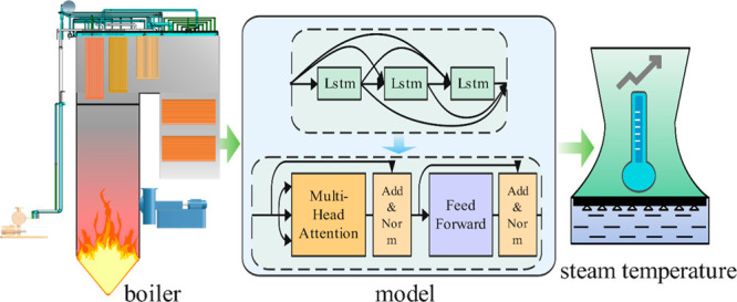
Flexible operation of large-scale boilers for electricity generation is essential in modern power systems. An accurate prediction of boiler steam temperature is of great importance to the operational efficiency of boiler units to prevent the occurrence of overtemperature. In this study, a dense, residual long short-term memory network (LSTM)-attention model is proposed for steam temperature prediction. In particular, the residual elements in the proposed model have a great advantage in improving the accuracy by adding short skip connections between layers. To provide overall information for the steam temperature prediction, uncertainty analysis based on the proposed model is performed to quantify the uncertainties in steam temperature variations. Our results demonstrate that the proposed method exhibits great performance in steam temperature prediction with a mean absolute error (MAE) of less than 0.6 °C. Compared to algorithms such as support-vector regression (SVR), ridge regression (RIDGE), the recurrent neural network (RNN), the gated recurrent unit (GRU), and LSTM, the prediction accuracy of the proposed model outperforms by 32, 16, 12, 10, and 11% in terms of MAE, respectively. According to our analysis, the dense residual LSTM-attention model is shown to provide an accurate early warning of overtemperature, enabling the development of real-time steam temperature control.
1. Introduction
The operational flexibility of large-scale boilers plays a critical role in today’s power systems with a large share of renewable energy sources.1,2 However, these boilers may face various issues such as overtemperature, slagging and corrosion of the walls, especially under load variations. Recently, scholars carried out a large number of studies on the use of data-driven models to monitor boiler operating parameters including the least-squares support vector (LSSV) model,3 support vector regression (SVR) model,4 autoregressive integrated moving average (ARIMA) model,5 and convolutional neural network (CNN) model.6 Romeo et al.7 established a model for biomass boiler monitoring with an artificial neural network (ANN). Combustion flue gas composition, staged heat transfer, and the slagging evolution index were predicted using this model. Sujatha et al.8 used a discriminant radial basis network combined with the boiler flame image collected by a charge coupled device (CCD) camera to monitor the combustion status of coal-fired boilers. Zeng et al.9 established a dynamic adaptive four-parameter discretegrey system model for coalbed methane production, and the mean relative percentage error was 0.48%. Yu et al.10 developed an algorithm based on the gray-predictor-based algorithm (GPBA) to monitor the uncertainty of steam flow and noise. Tong et al.11 proposed an online prediction program for the heating surface dust scale based on wavelet analysis and SVR. The prediction accuracy on the test data was 98.5%. Grochowalski et al.12 developed a CNN program to predict 12 temperature distributions in the boiler combustion chamber, including 48 input parameters, and compared and analyzed the differences between the 12 target predictions.
Stable boiler steam temperature changes can avoid overtemperature and tube burst accidents. However, the steam temperature delay characteristic is significant and extremely unstable with the change in working conditions. It is very difficult to accurately predict the temperature change. Mazalan et al.13 predicted the steam temperature of a boiler using a Levenberg–Marquardt learning algorithm combined with a neural network. The study found that the main factors of the steam temperature change in coal-fired power plants are generator output power, steam flow, steam pressure, and desuperheating water flow. However, the best machine learning model still suffers from poor stability and overfitting.
The influence of time on the prediction accuracy of the steam temperature cannot be ignored. The generation of the steam temperature has a significant delay characteristic. The long short-term memory network (LSTM) has good performance in time-series forecasting, which solves the problems of gradient disappearance, gradient explosion, and a long sequence dependence in the long sequence training process.14,15 Gupta et al.16 used a single layer of LSTM with 32 nodes to predict fouling in air preheaters, which can be predicted 3 months in advance. Tan et al.17 analyzed the effect of different delay time sequences on the model. Li et al.18 studied the comparison of different granularity windows based on LSTM and found that the LSTM network exhibited high performance in predicting both short term and long term, but the difference became larger for long-term prediction. Cheng et al.19 performed a sensitivity analysis based on LSTM to study the importance of multiple variables in the model. Chen et al.20 proposed a dynamic threshold estimation method to identify anomalous data and constructed performance metrics for key parameters on LSTM. Attention structures such as transformers have achieved great success in text translation and speech recognition. A hierarchical attention structure is proposed to improve the performance of CNN models.21 Li et al.22 introduced an attention mechanism to improve the performance of the the building energy consumption prediction, and their attention mechanism showed that key useful information was given greater weight. Inapakurthi et al.23 proposed a multiobjective evolutionary algorithm to realize the optimal network structural design of a recurrent neural network (RNN) and LSTM in univariate and multivariate environments and to improve the modeling accuracy using Monte Carlo global sensitivity analysis. This shows that intelligent algorithms achieve excellent results in network hyperparameter optimization.24−26 Uncertainty analysis is important compared to fixed value analysis because of uncertainties in data measurement, model fitting, and operating conditions. By considering the influence of multiple influencing factors to optimize the uncertain parameters, the validity of the uncertainty analysis is proven.27−29
Although machine learning models have achieved some success in many fields,30,31 research is still needed on boilers. Boiler combustion is complex but easily produces ash, resulting in large temperature changes and a large lag. Therefore, an accurate prediction of steam temperature is challenging. The prediction of boiler operating parameters has been a hot issue in recent years. However, the models based on time-series information are less frequently studied in boilers. To overcome the above shortcomings, a boiler steam temperature prediction model based on the dense residual LSTM-attention network is proposed to improve the prediction performance. In addition, a quantile-based dense residual LSTM-attention network interval prediction modeling method is proposed, which uses the boiler steam temperature prediction result interval instead of the traditional deterministic prediction result.
The rest of this study is organized as follows. Section 2 describes the coal-fired boiler model, experimental data, and proposed methodology in detail. Section 3 provides the results and a discussion of the proposed method for coal-fired boiler operating data. Conclusions and future work are given in Section 4.
2. Methodology
2.1. Coal-Fired Boiler
A real-scale coal-fired boiler is selected as the case study model. The furnace has a cross section of 7.09 m × 7.09 m, and the average flow velocity of flue gas is 8 m/s. Boiler combustion involves complex heat transfer and flow, and it easily generates a large amount of ash, which leads to large changes in steam temperature and long delay times.
As shown in Figure 1, the boiler in this case has a complete heat exchange process and multiple heating surface combinations. The pulverized coal enters the furnace through the burner, mixes with air, and burns to produce flue gas. Then, the flue gas passes through the panel superheater, a high-temperature superheater, a low-temperature superheater, and an economizer.
Figure 1.
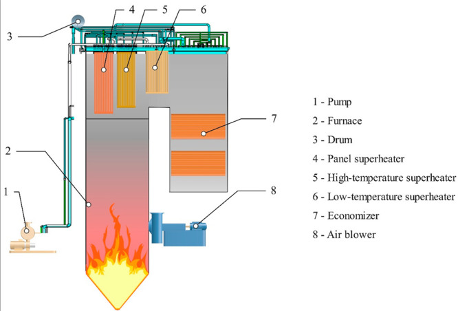
Model of the 170t/h tangential pulverized coal-fired boiler.
The final period of steaming requires multiple flue gas–water heat exchanges. As shown in Figure 2, the water enters the economizer, the steam drum, and the water wall through the feed pump and circulates back to the steam drum. Then, the steam flows through the low-temperature superheater, high-temperature superheater, and plate superheater to produce high-temperature steam. Changes in fuel and operating conditions can cause fluctuations in steam temperature. However, this process change requires a long delay time. Therefore, it is challenging to establish a time-series model to accurately predict changes in steam temperature.
Figure 2.

Schematics of the operation of a coal-fired boiler.
2.2. Experimental Data
The steam temperature from the boiler can be influenced by many factors. The studied data was collected by the distributed control system (DCS), including 69 variables such as steam flow, desuperheating water flow, boiler oxygen flow, blower air flow, and furnace outlet flue gas temperature. These 69 variables influence each other. For example, increasing the air volume of the blower will increase the temperature of the flue gas at the outlet of the furnace. High flue gas temperature leads to an increase in steam temperature. To maintain a stable temperature, the flow of desuperheating water is usually increased. These variables also affect the main steam temperature.
There are 3360 data samples in total. The sampling interval is 3 min, which covers 5 days of historical data for the studied boiler. Figure 3 and Table 1 show the temperature, flow, and pressure data of the main steam collected in this study. Figure 3 also indicates that the parameter change of the main steam is nonlinear and irregular. We chose the main steam temperature as the prediction target, and the temperature range is between 500.08 and 533.25 °C. In particular, the purpose of our results is to predict the main steam temperature changes in the future. The historical data of the main steam temperature can also be used as input variables in the model.
Figure 3.
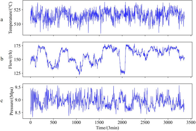
(a) Steam temperature data. (b) Steam flow data. (c) Steam pressure data.
Table 1. Steam Temperature Data Statistics.
| temperature | count | mean | max | min |
|---|---|---|---|---|
| data | 3360 | 519.08 °C | 533.25 °C | 500.08 °C |
We choose 15% of the total data as the test set and 85% of the total data as the training set. The data collection times of the test set and the training set do not overlap or leak. Specifically, we used a total of 2880 samples from 2019/5/24 0:00 to 2019/5/29 23:57 as the training set and a total of 480 samples from 2019/5/29 0:00 to 2019/5/30 23:57 as the test set. Because of the fluctuation and working characteristics of the sensor, missing values appear in the data. We fill in the missing values with the values from the previous moment and normalize the maximum and minimum values.
2.3. Dense Residual LSTM-Attention Network
Time-series forecasting has always been a challenging task. The recurrent neural network (RNN)32 is a time-series model that can effectively process sequence data. Many theories and experiments on the topic of RNN have been reported. Problems with RNN are encountered in practice, called “vanishing gradients” and “exploding gradients”.33,34 Because of the sequentially connected structure of the RNN, only recent states are considered. Training RNN becomes difficult when samples have long sequences of dependencies.
We propose a novel dense residual LSTM-attention network. As shown in Figure 4, it consists of two parts: an LSTM part and an attention part. The input [Xt,Xt–1,...,Xt–n] is an [n + 1, c] vector, where n + 1 represents the time dimension and c represents that the input at each time is a c variable. The input vector is dimensionally transformed by 1 × 1 convolution to obtain [n + 1, c′], where c′ is the transformed dimension. The obtained results are connected to the LSTM network part to extract features, and each layer of LSTM is [n + 1, c′]. The result output by LSTM is connected to the attention part to extract important feature components, the feature vector from the last time is selected, and the output dimension is [1, c′]. Finally, the [1, c′] dimensional vector is connected to the fully connected layer and outputs a k-dimensional vector [Yt+1,Yt+2,...,Yt+k].
Figure 4.

Framework of the dense residual LSTM-attention network.
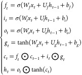
The residual connection exhibits good performance in the field of image recognition. Our work adds a multiple LSTM dense residual connection structure, and this design can reduce information loss and better capture more comprehensive information. Figure 5a is a structural diagram of LSTM. It controls the inflow and outflow of historical information through a gating design so as to avoid the disappearance of long-distance historical information. LSTM is composed of memory cells and three gated structures. Memory cells are used to store historical information; three gated structures include the forget gate, input gate, and output gate. They control the inflow and outflow of information through activation functions. Iterative formulas are used to extract timing-related features between gates. They are calculated using the follow equations.
 |
1 |
where σ represents the sigmoid activation function; tanh represents the double tangent activation function; W and U represents the weight matrix. Assuming the dimension of the LSTM cell input and output is m, the dimension of the weight matrix is [m, m]. b represents the bias matrix; ft, it, ot, gt, ct, and ht represent the forget gate, input gate, output gate, nonlinear transformation of the input, cell state, hidden state, respectively; and ⊙ represents elementwise multiplication.
Figure 5.
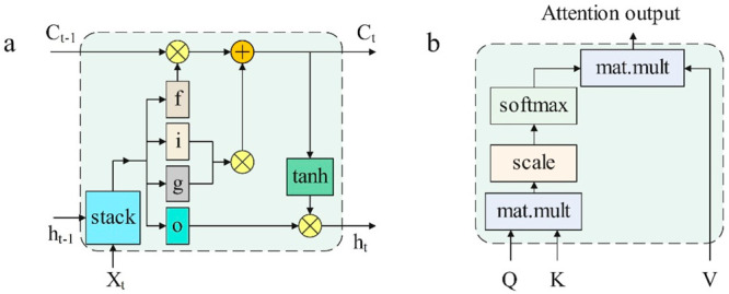
(a) Architecture of an LSTM cell. (b) Architecture of attention.
The attention part is a multihead attention structure. This design performs well in the fields of translation and text recognition. As shown in Figure 5b, it uses the query-key-value (Q–K–V) mode to output self-attention to the input sequence. It can extract the features of important regions. The attention parts can be connected to each other. Attention can be expressed in the following form
| 2 |
where Q is the query matrix, K is the key matrix, V is the value matrix, and dk is the hidden dimension of K. The dimension of input X is n, and Q, K, and V are is obtained by multiplying input X and parameter matrix W. The dimensions of Q, K, and V are [n, dk].
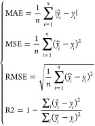
To evaluate the developed steam temperature prediction model, four evaluation indicators were introduced, namely, the mean absolute error (MAE), square root error (MSE), mean square root error (RMSE), and r-square (R2). The following equations are the definitions of the four evaluation indicators
 |
3 |
where yi is the actual value, ŷi is the predicted value, and n is the number of samples.
2.4. Method for Uncertainty Analysis
There are many uncertain factors in the boiler steam–water system. The final steam temperature has uncertain fluctuations. The reliability of results must be considered. Traditional deterministic prediction methods cannot give the quality of steam temperature prediction results. The uncertainty analysis method can give the confidence interval of the prediction result. This interval describes the possible range of future forecast results. More accurate forecasts are accompanied by lower uncertainty. Therefore, the realization of the interval prediction of the steam temperature helps boiler staff to understand the uncertainty and risk levels of future steam temperature changes.
We proposed an interval prediction modeling method based on the quantile and dense residual LSTM-attention network. It can effectively solve the problem of uncertainty prediction modeling of the boiler main steam temperature and estimate the quality of the prediction result of the steam temperature. Figure 6 shows the calculation process of uncertainty analysis. Quantile regression is used to study the relationship between the input X and the conditional quantile of the response variable Y, namely,
| 4 |
where τ is the quantile, the value is 0–1, β(τ) = [β0(τ), β1(τ), β2(τ), ...., βn(τ)]represents the quantile regression coefficient, which will change as the quantile changes, and n is the number of samples.
Figure 6.

Uncertainty analysis and calculation process.
The quantile regression coefficients β(τ) can be used to obtain the response of the input variable to the output variable in different quantiles. When τ takes continuous values in (0, 1), the conditional distribution of the response variable can be obtained, and then the conditional density can be obtained. Model training can be transformed into solving the following optimization problems:35
| 5 |
where yi is the actual value, Xi is the input, ŷi is the predicted value, τ is the quantile point, and β(τ) represents the quantile regression coefficient.
We divide the training set and validation set from the training data. The stopping criterion for model training is that the square root error of the validation set is less than the tolerance set of the algorithm or more than the maximum number of rounds, and the algorithm terminates.
To accurately and quantitatively perform uncertainty analysis, the quantile score (QS) and the prediction-interval-normalized root-mean-square width (PINRW) are used to evaluate the quality of probabilistic prediction results. QS can be expressed in the following form
 |
6 |
where τ is the quantile point, τi corresponds to the ith τ, r represents the number of τ values, N is the number of time points, yt is the actual value at time t, and ŷt(τi) is the predicted value at times t and τ. PINRW is an indicator of the width of the interval. It can be expressed in the following form
| 7 |
where α is the confidence and R is the range of samples. Utα is the upper bound of confidence at time t, and Lt is the lower bound of confidence at time t.
3. Results and Discussion
3.1. Performance of Different Models
In our experiments, we comprehensively compare the proposed model with SVR, ridge regression (RIDGE), RNN, the gated recurrent unit (GRU), and LSTM. For all models, we divided the training set and validation set from the training data for model training. We use 10-fold cross-validation to prevent the risk of overfitting. The optimal weights of the model on the validation set are selected to be validated on the test set. All of our experiments are repeated 10 times, and the mean values of the metrics are compared to remove the randomness of model training. For all models, the input historical time dimension is 5, the feature dimension for each historical time is constructed from data points of 69 variables, and the output dimension is 1. We applied a grid search to optimize the parameters of the SVR and RIDGE models. Parameters such as the learning rate and the number of nodes in each layer in the RNN, GRU, and LSTM models and our proposed model are the same and are set empirically and chosen by trial and error. All models are built on the pytorch platform. Additional details and control experiments are provided in Table 2.
Table 2. Parameter Settings of Comparative Experiments.
| model | parameters | quantity |
|---|---|---|
| SVR | c | 0–1 |
| gamma | 0–1 | |
| RIDGE | alpha | 0–1 |
| (RNN, GRU, LSTM) | number of layers | 3 |
| number of neurons in each layer | 64 | |
| learning rate | 0.001 | |
| number of iterations | 30 | |
| LSTM-attention | number of LSTM layers | 3 |
| number of neurons in each LSTM layer | 64 | |
| number of attention layers | 1 | |
| learning rate | 0.001 | |
| number of iterations | 30 |
Figure 7 is a comparison diagram of the predicted value and the true value of the dense residual LSTM-attention network. It can be seen that our method has a good predictive effect, and the curve of the predicted value and the actual value is very close. In the prediction of the next 3 min, the errors in the test set are almost all within ±5%.
Figure 7.
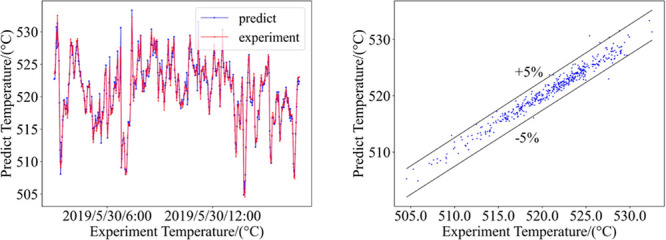
Prediction and experimental results for the next 3 min.
The predictive effects of different models are quantitatively analyzed. As shown in Table 3, compared with SVR, RIDGE, RNN, GRU, and LSTM, our method achieves competitive advantages on the four evaluation metrics for predicting the steam temperature in the next 3 min. Specifically, the error in our method for the mean absolute error (MAE) is 0.059, which indicates that the average error between the predicted value and the experimental value is within ±0.6 °C. Compared to SVR and RIDGE, the prediction accuracy of the proposed model outperforms those of SVR and RIDGE by 32% and that of MAE by 16%. SVR and RIDGE cannot extract the temporal features of variables, so they have poor predictive performance. The LSTM model error is 0.667 on MAE. However, our model has relative improvements of 12, 10, and 11% compared to the RNN, GRU, and LSTM models. This is because the residual elements and attention elements can obtain richer information. The closer the value of the r-square (R2) indicator to 1, the better. In addition, our model achieves the square root error (MSE), mean square root error (RMSE), and R2 metrics, providing better prediction performance.
Table 3. Comparison of Our Proposed Model with Different Models.
| model | MAE | MSE | RMSE | R2 |
|---|---|---|---|---|
| SVR | 0.875 | 1.300 | 1.140 | 0.947 |
| RIDGE | 0.710 | 0.951 | 0.975 | 0.961 |
| RNN | 0.681 | 0.876 | 0.936 | 0.964 |
| GRU | 0.662 | 0.825 | 0.908 | 0.966 |
| LSTM | 0.667 | 0.828 | 0.910 | 0.966 |
| LSTM-attention | 0.596 | 0.714 | 0.845 | 0.971 |
3.2. Parametric Analysis
To analyze the prediction performance of the model in more detail, we analyzed the prediction effect of the long-term horizon and the feature importance analysis.
3.2.1. Long-Term Horizon
As shown in Figure 8, we compare the effect of different prediction durations 3–30 min ahead. It can be seen that the prediction performance of our model is the best for both short-term and long-term predictions. Compared to SVR, RIDGE, RNN, GRU, and LSTM, our model improves by 29, 26, 19, 15, and 17% in terms of average MAE from 3 to 30 min. The prediction accuracy decreases as the prediction time increases. For example, forecasting 3 min ahead provides better performance than forecasting 6 min ahead. This is because when the advance prediction time increases, the steam temperature of the boiler fluctuates greatly, which increases the difficulty of prediction. Compared to the LSTM model, our model is 11% lower in MAE, 14% lower in MSE, and 7% lower in RMSE in predicting temperature 3 min ahead. Meanwhile, our model is 13% lower in MAE, 30% lower in MSE, and 17% lower in RMSE in predicting temperature 15 min ahead. This shows that our model is more advantageous in predicting long-term time series, but when forecasting 15–30 min in advance, all model errors are large. To obtain accurate results, it is recommended that the prediction time be less than 15 min.
Figure 8.

Error of prediction 3–30 min into the future.
3.2.2. Feature Importance Analysis
We conduct an experimental analysis on the predictive importance of the characteristics of the model variables. The shapley additive explanations (SHAP) method was used to calculate the variable’s contribution to the predicted target value,36 which is important for model interpretability. SHAP provides key parameters that affect the target and whether the contribution of input features is positive or negative. As shown in Figure 9, a positive value of the shape value indicates a positive correlation, and a negative value indicates a negative correlation. The darker the red, the greater the importance. It can be seen that the historical main steam temperature and header temperature are positively correlated with the predicted target, and the desuperheating water flow rate is negatively correlated with the predicted target. The desuperheating water flow, historical main steam temperature, and header temperature are the main factors that affect the predicted steam temperature target. Changes in these important variables should be noted when monitoring the boiler steam temperature. This helps to regulate the steam temperature and quickly locate the cause of overtemperature faults.
Figure 9.
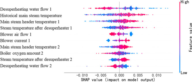
Description of the importance of different features for a 3 min step ahead prediction.
3.3. Uncertainty Analysis Results
On the basis of the quantile and dense residual LSTM-attention model, we predicted the boiler steam temperature interval. As shown in Figure 10, the lower uncertainty has a narrower forecast fluctuation range, which means that the quality of the forecast results is more accurate. For a forecast 3 min ahead, the range of uncertainty is small. However, comparing the prediction intervals of different time steps in the future, as the future prediction time increases, the fluctuation range of the prediction interval becomes larger. For example, the uncertainty interval of the forecast 18 min ahead is large, which means that the quality of the forecast results decreases.
Figure 10.
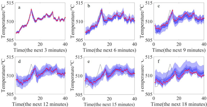
(a–f) Different confidence intervals predictions for the range of 3–18 min, with the the median value in red and the experimental value in black. The colors of different intervals represent the prediction results under different confidence levels.
As shown in Table 4, the influence of the prediction step size on the prediction performance in the uncertainty interval is quantitatively analyzed in terms of QS and PINRW. QS is an indicator of the quantitative analysis of the interval prediction error. PINRW represents the average widths of prediction intervals. A good interval prediction result should be shortened with a small average width of the prediction interval and a location close to the experimental value. It can be seen that the prediction time increases from 3 to 18 min and that QS increases by 81%. Furthermore, PINRW decreases as the confidence interval decreases from 90 to 60%. This shows that the model can obtain the effective lower and upper bounds of the prediction results. Therefore, uncertainty analysis provides more comprehensive information for the prediction results and helps to judge the reliability of the model prediction results.
Table 4. Comparison of Uncertain Quantitative Indicators for the Range of 3–18 min.
| future time (min) | QS/°C | PINRW (90%) | PINRW (80%) | PINRW (70%) | PINRW (60%) |
|---|---|---|---|---|---|
| 3 | 0.3017 | 0.1261 | 0.0837 | 0.0555 | 0.0163 |
| 6 | 0.7694 | 0.3355 | 0.1171 | 0.1000 | 0.1395 |
| 9 | 1.0127 | 0.5368 | 0.2360 | 0.1461 | 0.1453 |
| 12 | 1.2665 | 0.4624 | 0.3063 | 0.1831 | 0.0708 |
| 15 | 1.4107 | 0.4584 | 0.2568 | 0.2257 | 0.0989 |
| 18 | 1.6279 | 0.4846 | 0.2925 | 0.2146 | 0.1434 |
4. Conclusions
In this study, we propose a dense residual LSTM-attention model to predict boiler steam temperature. Our model establishes a relationship between variables such as desuperheating water flow, amount of boiler oxygen, and the target change in steam temperature. The model is evaluated by using the operating data of a real boiler, and the results show that the proposed model is effective. According to our analysis, our model has the following advantages: (1) Compared to SVR, RIDGE, RNN, GRU, and LSTM methods, our method can achieve better performance in forecasting. In the target prediction of the next 3 min, the mean absolute error of our method with respect to the test data is within ±0.6 °C. (2) Compared to the prediction effect of the model at multiple different future times, the results show that our model can predict long-term time series well. Meanwhile, a prediction horizon of less than 15 min is suggested for steam temperature prediction. (3) Different variable features have different degrees of importance in the dense residual LSTM-attention model. Parameters such as the desuperheating water flow, historical main steam temperature, and header temperature are the main factors that affect the prediction results of the steam temperature. (4) We have proposed an interval uncertainty analysis method, which can give the fluctuation interval of the result and provide comprehensive information for boilers.
The research results are of great significance for fault early warning and energy efficiency improvement and can also be applied to multivariate time series problems such as solar power generation steam temperature predictions and wind power uncertainty analysis. Future work will focus on combining the proposed prediction model with an operational control strategy for effective boiler operation.
Acknowledgments
This research was funded by the National Natural Science Foundation of China (52075481) and the Zhejiang Provincial Natural Science Foundation (LD21E050003).
The authors declare no competing financial interest.
References
- D’Ettorre F.; De Rosa M.; Conti P.; Testi D.; Finn D. Mapping the energy flexibility potential of single buildings equipped with optimally-controlled heat pump, gas boilers and thermal storage. Sust. Cities Soc. 2019, 50, 101689. 10.1016/j.scs.2019.101689. [DOI] [Google Scholar]
- Li Y.; Tong Z. Development of real-time adaptive model-free extremum seeking control for CFD-simulated thermal environment. Sust. Cities Soc. 2021, 74, 103166. 10.1016/j.scs.2021.103166. [DOI] [Google Scholar]
- Yang T.; Ma K.; Lv Y.; Bai Y. Real-time dynamic prediction model of NOx emission of coal-fired boilers under variable load conditions. Fuel 2020, 274, 117811. 10.1016/j.fuel.2020.117811. [DOI] [Google Scholar]
- Wei Z.; Li X.; Xu L.; Cheng Y. Comparative study of computational intelligence approaches for NOx reduction of coal-fired boiler. Energy 2013, 55, 683–692. 10.1016/j.energy.2013.04.007. [DOI] [Google Scholar]
- Tunckaya Y.; Koklukaya E. Comparative prediction analysis of 600 MWe coal-fired power plant production rate using statistical and neural-based models. J. Energy Inst. 2015, 88 (1), 11–18. 10.1016/j.joei.2014.06.007. [DOI] [Google Scholar]
- Dhanuskodi R.; Kaliappan R.; Suresh S.; Anantharaman N.; Arunagiri A.; Krishnaiah J. Artificial Neural Networks model for predicting wall temperature of supercritical boilers. Appl. Therm. Eng. 2015, 90, 749–753. 10.1016/j.applthermaleng.2015.07.036. [DOI] [Google Scholar]
- Romeo L. M.; Gareta R. Neural network for evaluating boiler behaviour. Appl. Therm. Eng. 2006, 26 (14), 1530–1536. 10.1016/j.applthermaleng.2005.12.006. [DOI] [Google Scholar]
- Sujatha K.; Pappa N. Combustion monitoring of a water tube boiler using a discriminant radial basis network. ISA Trans. 2011, 50 (1), 101–110. 10.1016/j.isatra.2010.08.006. [DOI] [PubMed] [Google Scholar]
- Zeng B.; Li H. Prediction of Coalbed Methane Production in China Based on an Optimized Grey System Model. Energy Fuels 2021, 35 (5), 4333–4344. 10.1021/acs.energyfuels.0c04195. [DOI] [Google Scholar]
- Yu N.; Ma W.; Su M. Application of adaptive Grey predictor based algorithm to boiler drum level control. Energy Convers. Manage. 2006, 47 (18), 2999–3007. 10.1016/j.enconman.2006.03.035. [DOI] [Google Scholar]
- Tong S.; Zhang X.; Tong Z.; Wu Y.; Tang N.; Zhong W. Online Ash Fouling Prediction for Boiler Heating Surfaces based on Wavelet Analysis and Support Vector Regression. Energies 2020, 13 (1), 59. 10.3390/en13010059. [DOI] [Google Scholar]
- Grochowalski J.; Jachymek P.; Andrzejczyk M.; Klajny M.; Widuch A.; Morkisz P.; Hernik B.; Zdeb J.; Adamczyk W. Towards application of machine learning algorithms for prediction temperature distribution within CFB boiler based on specified operating conditions. Energy 2021, 237, 121538. 10.1016/j.energy.2021.121538. [DOI] [Google Scholar]
- Mazalan N. A.; Malek A. A.; Wahid M. A.; Mailah M.; Saat A.; Sies M. M. Main Steam Temperature Modeling Based on Levenberg-Marquardt Learning Algorithm. Appl. Mech. Mater. 2013, 388, 307–311. 10.4028/www.scientific.net/AMM.388.307. [DOI] [Google Scholar]
- Dong Y.; Zhang Y.; Liu F.; Cheng X. Reservoir Production Prediction Model Based on a Stacked LSTM Network and Transfer Learning. ACS Omega 2021, 6 (50), 34700–34711. 10.1021/acsomega.1c05132. [DOI] [PMC free article] [PubMed] [Google Scholar]
- Fernández-Llaneza D.; Ulander S.; Gogishvili D.; Nittinger E.; Zhao H.; Tyrchan C. Siamese Recurrent Neural Network with a Self-Attention Mechanism for Bioactivity Prediction. ACS Omega 2021, 6 (16), 11086–11094. 10.1021/acsomega.1c01266. [DOI] [PMC free article] [PubMed] [Google Scholar]
- Gupta A.; Jadhav V.; Patil M.; Deodhar A.; Runkana V.. Forecasting of Fouling in Air Pre-Heaters Through Deep Learning. ASME 2021 Power Conference, 2021.
- Tan P.; He B.; Zhang C.; Rao D.; Li S.; Fang Q.; Chen G. Dynamic modeling of NOX emission in a 660 MW coal-fired boiler with long short-term memory. Energy 2019, 176, 429–436. 10.1016/j.energy.2019.04.020. [DOI] [Google Scholar]
- Li Y.; Tong Z.; Tong S.; Westerdahl D. A data-driven interval forecasting model for building energy prediction using attention-based LSTM and fuzzy information granulation. Sust. Cities Soc. 2022, 76, 103481. 10.1016/j.scs.2021.103481. [DOI] [Google Scholar]
- Cheng W.; Zhang Y.; Wang P. Effect of spatial distribution and number of raw material collection locations on the transportation costs of biomass thermal power plants. Sust. Cities Soc. 2020, 55, 102040. 10.1016/j.scs.2020.102040. [DOI] [Google Scholar]
- Chen H.; Liu H.; Chu X.; Liu Q.; Xue D. Anomaly detection and critical SCADA parameters identification for wind turbines based on LSTM-AE neural network. Renewable Energy 2021, 172, 829–840. 10.1016/j.renene.2021.03.078. [DOI] [Google Scholar]
- Jin I.; Nam H. HiDRA: Hierarchical Network for Drug Response Prediction with Attention. J. Chem. Inf. Model. 2021, 61 (8), 3858–3867. 10.1021/acs.jcim.1c00706. [DOI] [PubMed] [Google Scholar]
- Li G.; Zhao X.; Fan C.; Fang X.; Li F.; Wu Y. Assessment of long short-term memory and its modifications for enhanced short-term building energy predictions. J. Build. Eng. 2021, 43, 103182. 10.1016/j.jobe.2021.103182. [DOI] [Google Scholar]
- Inapakurthi R. K.; Miriyala S. S.; Mitra K. Deep learning based dynamic behavior modelling and prediction of particulate matter in air. Chem. Eng. J. 2021, 426, 131221. 10.1016/j.cej.2021.131221. [DOI] [Google Scholar]
- Inapakurthi R. K.; Miriyala S. S.; Mitra K. Recurrent neural networks based modelling of industrial grinding operation. Chem. Eng. Sci. 2020, 219, 115585. 10.1016/j.ces.2020.115585. [DOI] [Google Scholar]
- Liang R.; Chang X.; Jia P.; Xu C. Mine Gas Concentration Forecasting Model Based on an Optimized BiGRU Network. ACS Omega 2020, 5 (44), 28579–28586. 10.1021/acsomega.0c03417. [DOI] [PMC free article] [PubMed] [Google Scholar]
- Zhang Q.; Tong Z.; Tong S.; Cheng Z. Modeling and dynamic performance research on proton exchange membrane fuel cell system with hydrogen cycle and dead-ended anode. Energy 2021, 218, 119476. 10.1016/j.energy.2020.119476. [DOI] [Google Scholar]
- Virivinti N.; Hazra B.; Mitra K. Optimizing grinding operation with correlated uncertain parameters. Mater. Manuf. Processes 2021, 36 (6), 713–721. 10.1080/10426914.2020.1854473. [DOI] [Google Scholar]
- Sharma S.; Pantula P. D.; Miriyala S. S.; Mitra K. A novel data-driven sampling strategy for optimizing industrial grinding operation under uncertainty using chance constrained programming. Powder Technol. 2021, 377, 913–923. 10.1016/j.powtec.2020.09.024. [DOI] [Google Scholar]
- Inapakurthi R. K.; Pantula P. D.; Miriyala S. S.; Mitra K. Data driven robust optimization of grinding process under uncertainty. Mater. Manuf. Processes 2020, 35 (16), 1870–1876. 10.1080/10426914.2020.1802042. [DOI] [Google Scholar]
- Tong Z.; Miao J.; Tong S.; Lu Y. Early prediction of remaining useful life for Lithium-ion batteries based on a hybrid machine learning method. Journal of Cleaner Production 2021, 317, 128265. 10.1016/j.jclepro.2021.128265. [DOI] [Google Scholar]
- Tong Z.; Xin J.; Ling C. Many-Objective Hybrid Optimization Method for Impeller Profile Design of Low Specific Speed Centrifugal Pump in District Energy Systems. Sustainability 2021, 13 (19), 10537. 10.3390/su131910537. [DOI] [Google Scholar]
- Schuster M.; Paliwal K. K. Bidirectional recurrent neural networks. IEEE Trans. Signal Process. 1997, 45 (11), 2673–2681. 10.1109/78.650093. [DOI] [Google Scholar]
- Hochreiter S.; Bengio Y.; Frasconi P.; Schmidhuber J.. Gradient flow in recurrent nets: the difficulty of learning long-term dependencies. A Field Guide to Dynamical Recurrent Neural Networks; IEEE Press: 2001. [Google Scholar]
- Pascanu R.; Mikolov T.; Bengio Y.. On the difficulty of training recurrent neural networks. International Conference on Machine Learning; PMLR, 2013; pp 1310–1318.
- Zhang W.; Quan H.; Srinivasan D. An Improved Quantile Regression Neural Network for Probabilistic Load Forecasting. IEEE Trans. Signal Process. 2019, 10 (4), 4425–4434. 10.1109/TSG.2018.2859749. [DOI] [Google Scholar]
- Mangalathu S.; Hwang S.-H.; Jeon J.-S. Failure mode and effects analysis of RC members based on machine-learning-based SHapley Additive exPlanations (SHAP) approach. Eng. Struct. 2020, 219, 110927. 10.1016/j.engstruct.2020.110927. [DOI] [Google Scholar]