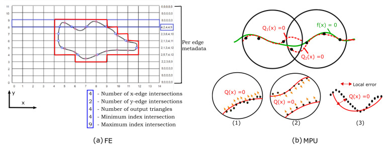
Figure 2.

FE and MPU: (a) The region of the FE grid processed at the end of the second stage; on the right side is a metadata array describing the interaction of the isosurface with the grid edges. (b) Principle of MPU. Top: Two local approximations (dashed red curves) blended to form the global MPU function (solid green curve). Bottom: (1–2) quadric functions are used to approximate the local shape; (1) bivariate quadric is used; (2) general 3D quadric is used; (3) the local function’s error is evaluated in each step of the algorithm in order to determine if the local function has to be refined.