Fig. 2.

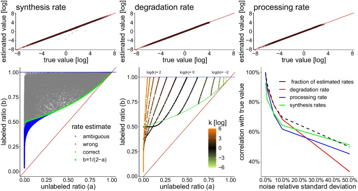
Simulated data. Top row: the method correctly estimates synthesis, processing and degradation rates. Points with ambiguous solutions are not shown. Some points corresponding to high rates cannot be estimated correctly as the system as already reached steady state during the simulated “pulse’. Bottom left: the measurement space can be partitioned into ambiguous and unambiguous regions. The green line corresponds to $b=\frac{1}{2-a}$. Above that line, rates are correctly and unambiguously estimated. Boundary cases are sometimes wrongly estimated, probably due to numerical errors (red dots). Bottom center: Trajectories in the phase space are solely determined by the k parameter. They start at time $T=0$ at the top ($b=1$) and go down. For $k<1$ the trajectories (in olive) remain above the green line defined by $b={(2-a)}^{-1}$ and do not cross. For $k>1$ (in orange), they cross each other below the green line. The velocity at which the system follows the trajectory depends on the actual values of $\beta$ and $\gamma$. Bottom right: effect of adding simulated Gaussian noise to the exon and intron quantifications on the correlation between estimated and true values of the rates. The abscissa indicates the standard deviation of the noise relative to the expression value. The black dashed line indicates the fraction of transcripts for which rates could be estimated. For example, a 10% standard deviation for noise, provides rates for about 70% of transcripts with around 62%-68% correlation with the true values