The unit-Weibull distribution as an alternative to the Kumaraswamy distribution for the modeling of quantiles conditional on covariates

ABSTRACT

The Beta distribution is the standard model for quantifying the influence of covariates on the mean of a response variable on the unit interval. However, this well-known distribution is no longer useful when we are interested in quantifying the influence of such covariates on the quantiles of the response variable. Unlike Beta, the Kumaraswamy distribution has a closed-form expression for its quantile and can be useful for the modeling of quantiles in the absence/presence of covariates. As an alternative to the Kumaraswamy distribution for the modeling of quantiles, in this paper the unit-Weibull distribution was considered. This distribution was obtained by the transformation of a random variable with Weibull distribution. The same transformation applied to a random variable with Exponentiated Exponential distribution generates the Kumaraswamy distribution. The suitability of our proposal was demonstrated to model quantiles, conditional on covariates, with two simulated examples and three real applications with datasets from health, accounting and social science. For such data sets, the obtained fits of the proposed regression model were compared with those provided by the Beta and Kumaraswamy regression models.

1. Introduction

In applied statistics, it is very common to deal with the uncertainty of a bounded phenomenon. In several fields of knowledge, we often encounter variables like proportions of a certain characteristic, scores of some ability tests, different indices and rates, which lie on the interval $(0,1)$, see, for instance, [9,11,20,24,26,41,49], among other applications. In such situations, continuous probability distributions with domain on $(0,1)$ interval are crucial to probabilistic modeling of the phenomena. When covariates are associated with the response of a continuous response on the unit interval, the Beta regression model, introduced by Cepeda-Cuervo [7] and Ferrari and Cribari-Neto [14], is the most widely used model, mainly because of its flexibility and direct parameter interpretation. In this model, the regression parameters are interpretable in terms of the mean, being the model intrinsically heteroscedastic accommodating asymmetries [12].

Although the Beta distribution is flexible to fit data on the unit interval, other distributions on the unit interval have been proposed in the literature, such as the Johnson $S_B$ distribution [25], the unit-Gamma distribution [18,50], the Kumaraswamy distribution [28], the unit-Logistic distribution [51], the simplex distribution [4], the Beta rectangular distribution [21], among others. These mentioned distributions were extended to explain the behavior of the response variable in the presence of covariates. For instance, it is possible to refer the simplex regression model [4], the Beta rectangular regression model [6], the Kumaraswamy regression model [5,37], the Johnson $S_B$ regression model [33], the unit-Gamma regression model [38], the unit-Logistic regression model [13], the Log-Lindley regression model [17] and the unit-Lindley regression model [35].

Recently, a new probability distribution, called the unit-Weibull distribution, with support on the unit interval, was proposed by Mazucheli et al. [36]. The authors derived several structural properties and showed that the distribution is very flexible and is highly competitive to many classical distributions on the unit interval. In contrast to the Beta distribution, the unit-Weibull distribution has a closed-form expression for the quantile function.

In this paper, we shall formulate a quantile regression model considering a parametrization of the unit-Weibull distribution in terms of the τth quantile. By reparameterizing the unit-Weibull distribution in terms of its quantile function, one gets the interpretation of its location parameter as being the τth quantile of the distribution. The strategy of reparametrizing the probability distribution as a function of quantile was considered by Mitnik and Baek [37] and Bayes et al . [5] to formulate the Kumaraswamy quantile regression model. Also, a fully parametric approach to quantile regression which treats both, the dependence on a single covariate and the random component parametrically, whose conditional distribution is modeled by the Generalized Gamma distribution was considered by Noufaily [40] and Noufaily and Jones [39].

It is well-known that there are at least three approaches to modeling quantiles conditional on covariates (i) the distribution-free (semiparametric) approach; (ii) the approach based on a pseudo-likelihood through an asymmetric Laplace distribution, or a mixture distribution and (iii) the parametric approach with traditional maximum likelihood framework. The current manuscript is classified as the third category.

As discussed in the statistical literature [see, for example, 5,27,37,43,54] the quantile regression analysis has been used in several contexts and its main advantage, when compared with the conditional-mean regressions, such as Beta regression, is that it provides a complete view of the conditional distribution by studying distinct quantiles. By employing quantile regression, such as conditional-median regressions, practitioners will have a more robust model for outliers than the usual Beta regression. Another advantage lies on the fact that if the conditional dependent variable is skewed, the median may be more appropriate when compared with the mean.

It is important to point out that the usual quantile regression is able to approximate the conditional quantiles of a response variable in the unit interval, by ways of the equivariance principle. Some relevant literature are [15,16,47,48] and references therein.

The remainder of this paper is organized as follows. Section 2 contains a brief description of the unit-Weibull distribution, some of its main properties and a new parametrization is introduced. The unit-Weibull quantile regression model and parameters estimation are described in Section 3, where we also presented a residual analysis to asses departure from the underlying distribution. In Section 4, a simulation study is conducted to evaluate finite sample behavior of the maximum likelihood estimators. Three real applications are presented in Section 5 using the proposed quantile regression model and other well-known regression models. The paper closes with some discussions and directions for future extensions.

2. The unit-Weibull distribution

Using the transformation $Y={\mathrm{e}}^{-X}$, where X follows the two-parameter generalized exponential distribution [19], we obtain the Kumaraswamy distribution [28]. Similarly, if X follows the two-parameter Weibull distribution [53] with probability density function (p.d.f.)

$$g(x\mid \alpha ,\mathrm{\text{β}})=\alpha \mathrm{\text{β}}{x}^{\mathrm{\text{β}}-1}{\mathrm{e}}^{-\alpha x^{\mathrm{\text{β}}}},x>0,\alpha ,\mathrm{\text{β}}>0,$$ (1)

we obtain the unit-Weibull (UW) distribution [36] with p.d.f.

$$f(y\mid \alpha ,\mathrm{\text{β}})=\frac{1}{y}\alpha \mathrm{\text{β}}(-\log y{)}^{\mathrm{\text{β}}-1}\exp \left[-\alpha (-\log y{)}^{\mathrm{\text{β}}}\right],0<y<1,$$ (2)

and cumulative distribution function (c.d.f.) given by

$$F(y\mid \alpha ,\mathrm{\text{β}})=\exp \left[-\alpha (-\log y{)}^{\mathrm{\text{β}}}\right],0<y<1,$$ (3)

where $\alpha >0$ and $\mathrm{\text{β}}>0$ are shape parameters. Special cases of the UW distributions include: the standard uniform distribution over the interval (0,1) ($\alpha =\mathrm{\text{β}}=1$), the power function distribution ($\mathrm{\text{β}}=1$) and the unit-Rayleigh distribution ($\mathrm{\text{β}}=2$). Therefore, the new distribution has connection with some well-known distributions, and hence, it can be very useful in many practical situations.

Since it is not possible to obtain a simple analytic expressions for $\mathbb{E}\left(Y\right),$ it is difficult to model the mean of Y in the absence/presence of covariates. On the other hand, the quantile function of the UW distribution has a simple analytic expression given by

$$Q(\tau \mid \alpha ,\mathrm{\text{β}})=\exp \left[-{\left(-\frac{\log \tau }{\alpha }\right)}^{1/\mathrm{\text{β}}}\right],0<\tau <1.$$ (4)

In order to introduce a quantile regression model, we shall re-parametrize (2) in terms of the τth quantile $\mu =Q(\tau \mid \alpha ,\mathrm{\text{β}})$ such that α can be written as follows:

$$\alpha =-\frac{\log \tau }{{\left(-\log \mu \right)}^{\mathrm{\text{β}}}}.$$ (5)

Under this parametrization, the p.d.f. and c.d.f. of the UW distribution can be written, respectively, as follows:

$$f(y\mid \mu ,\mathrm{\text{β}},\tau )=\frac{\mathrm{\text{β}}}{y}\left(\frac{\log \tau }{\log \mu }\right){\left(\frac{\log y}{\log \mu }\right)}^{\mathrm{\text{β}}-1}{\tau }^{(\log y/\log \mu {)}^{\mathrm{\text{β}}}},0<y<1$$ (6)

and

$$F(y\mid \mu ,\mathrm{\text{β}},\tau )={\tau }^{(\log y/\log \mu {)}^{\mathrm{\text{β}}}},0<y<1.$$ (7)

Hereafter, we shall use the notation $Y\sim \mathrm{U}\mathrm{W}(\mu ,\mathrm{\text{β}};\tau )$ where $\mu \in (0,1)$ is the quantile parameter, $\mathrm{\text{β}}>0$ is the shape parameter and $\tau \in (0,1)$ is assumed as known.

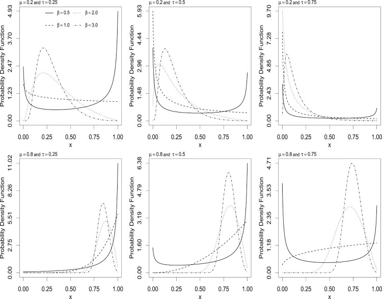
Figure 1 shows some possible shapes of the p.d.f. of the UW distribution for selected values of the parameters μ, β and τ. Note that the p.d.f. can assume different shapes (decreasing, increasing, unimodal, anti-unimodal) according to the values of its parameters. This shape flexibility makes UW distribution suitable for the data analysis on the unit interval. Furthermore, since μ is the τth quantile of the distribution of Y, it is a location parameter on the unit interval.

Figure 1.

Probability density function of the UW distribution for selected values of μ, β and τ.

The behavior of (6), for different values of μ, β and τ, can be studied considering it on the logarithmic scale. Note that

$$\frac{\mathrm{d}}{\mathrm{d}y}\log f\left(y\mid \mu ,\mathrm{\text{β}},\tau \right)=-\frac{1}{y}+\frac{\mathrm{\text{β}}-1}{y\log \left(y\right)}+\frac{{\mathrm{\text{β}}}^2\log \left(y\right)\log \left(\tau \right)}{\mathrm{\text{β}}\log \left(\mu \right)y\log \left(y\right)}$$ (8)

cannot be solved analytically in y. However, for $\mathrm{\text{β}}=1$ we have

$$\frac{\mathrm{d}}{\mathrm{d}y}\log f(y,\mid \mu ,\mathrm{\text{β}},\tau )=-\frac{1}{y}+\frac{\log \left(\tau \right)}{y\log \left(\mu \right)}$$ (9)

which guarantees that (6) is an increasing function in y if $\mu <\tau$ and a decreasing function in y if $\mu >\tau$. For $\mathrm{\text{β}}>1$ we have

$$\frac{{\mathrm{d}}^2}{\mathrm{d}{y}^2}\log f(y\mid \mu ,\mathrm{\text{β}},\tau )=A\left(y\right)\left\{\mathrm{\text{β}}\log \left(\tau \right)B\left(y\right)C\left(y\right)+2\log \left(y\right)+\left(1-\mathrm{\text{β}}\right)\left[1+\log \left(y\right)\right]\right\},$$ (10)

where $A\left(y\right)=1/y^2\log (y{)}^2$, $B\left(y\right)=[\mathrm{\text{β}}-\log (y)-1]$ and $C\left(y\right)=[\log (y)-\log (\mu ){]}^{\mathrm{\text{β}}}$.

In this case, for all $0<\mu ,\tau <1$ and 0<y<1, we have $A\left(y\right),B\left(y\right),C\left(y\right)>0$. Thus, the sign of (10) is always negative which implies that (6) is unimodal for all $0<\mu ,\tau <1$ and $\mathrm{\text{β}}>1$. On other hand, for $0<\mathrm{\text{β}},\tau ,\mu <1$ and $0<y<1$, we have $A\left(y\right),C\left(y\right)>0$ and $B\left(y\right)<0$. Thus, the sign of (10) is always positive which implies that (6) is bathhub for all $0<\mathrm{\text{β}},\mu ,\tau <1$.

3. The unit-Weibull quantile regression model

Considering the re-parametrized p.d.f (6), we can formulate a quantile regression model as in [5,37] where they considered for the Kumaraswamy distribution.

Let $Y_1,\dots ,Y_n$ be n independent random variables, where each $Y_i,i=1,\dots ,n,$ follows the p.d.f. in (6) with unknown quantile parameter ${\mu }_i$, unknown shape parameter β and $\tau \in (0,1)$ is assumed as known, that is, $Y_i\sim \mathrm{U}\mathrm{W}({\mu }_i,\mathrm{\text{β}};\tau )$. Here the UW quantile regression model is defined imposing that the quantile ${\mu }_i$ of $Y_i$ satisfies the following functional relation:

$$g\left({\mu }_i\right)={\mathit{\delta }}^{\mathrm{\top }}{\mathbf{x}}_i,i=1,\dots ,n,$$ (11)

where $\mathit{\delta }=({\delta }_0,\dots ,{\delta }_{p-1}{)}^{\mathrm{\top }}$ is a p-dimensional vector of unknown regression coefficients ($p<n$) and ${\mathbf{x}}_i=(1,x_{i1},\dots ,x_{i(p-1)}{)}^{\mathrm{\top }}$ denotes the observations on p known covariates. We shall assume that the quantile link function $g(\cdot )$ is a strictly increasing and twice differentiable function that maps $(0,1)$ into $\mathbb{R}$. There are several possibilities for the link function $g(\cdot )$. For instance, the most useful well-known link functions are:

1. $\mathrm{l}\mathrm{o}\mathrm{g}\mathrm{i}\mathrm{t}$: $g\left({\mu }_i\right)=\log \left({\mu }_i/\right(1-{\mu }_i\left)\right)$;

2. $\mathrm{p}\mathrm{r}\mathrm{o}\mathrm{b}\mathrm{i}\mathrm{t}$: $g\left({\mu }_i\right)={\mathrm{\Phi }}^{-1}\left({\mu }_i\right)$, where ${\mathrm{\Phi }}^{-1}(\cdot )$ is the standard normal quantile function;

3. complementary log-log: $g\left({\mu }_i\right)=\log [-\log (1-{\mu }_i\left)\right]$.

Due to the direct interpretation of the parameters in terms of odds, in this paper we consider only the logit link. Its interpretation when ${\mu }_i$ is the mean of the Beta distribution is given in [14]. When ${\mu }_i$ is the τth quantile, $0<\tau <1$, the interpretations are straightforward. In addition, a strictly positive link function relating the shape parameter β with covariates ${\mathbf{w}}_i$, not necessarily equal to ${\mathbf{x}}_i$, can be considered. Of course, other link functions might be explored.

3.1. Estimation

Let $Y_1,\dots ,Y_n$ be n independent random variables $Y_i\sim \mathrm{U}\mathrm{W}({\mu }_i,\mathrm{\text{β}};\tau )$ where

$${\mu }_i=\frac{\exp \left({\mathit{\delta }}^{\mathrm{\top }}{\mathbf{x}}_i\right)}{1+\exp \left({\mathit{\delta }}^{\mathrm{\top }}{\mathbf{x}}_i\right)},i=1,\dots ,n,$$

under the logit link function. For given $\tau \in (0,1),$ let $\mathit{\theta }=({\mathit{\delta }}^{\mathrm{\top }},\mathrm{\text{β}}{)}^{\mathrm{\top }}$ be the vector of p + 1 unknown parameters to be estimated using the method of maximum likelihood.

Using the form of the p.d.f. (6), the log-likelihood function is given by

$$\begin{array}{rl}\ell \left(\mathit{\theta }\right)& =\sum _{i=1}^n\log \left(\frac{\mathrm{\text{β}}}{y_i}\right)+\sum _{i=1}^n\log \left(\frac{\log \tau }{\log {\mu }_i}\right)+(\mathrm{\text{β}}-1)\sum _{i=1}^n\log \left(\frac{\log y_i}{\log {\mu }_i}\right)\\ & +\log \left(\tau \right)\sum _{i=1}^n{\left(\frac{\log y_i}{\log {\mu }_i}\right)}^{\mathrm{\text{β}}}.\end{array}$$ (12)

The maximum likelihood estimate (MLE) $\hat{\mathit{\theta }}=({\hat{\mathit{\delta }}}^{\mathrm{\top }},\widehat{\mathrm{\text{β}}}{)}^{\mathrm{\top }}$ of $\mathit{\theta }=({\mathit{\delta }}^{\mathrm{\top }},\mathrm{\text{β}}{)}^{\mathrm{\top }}$ is obtained by the maximizing log-likelihood function $\ell \left(\mathit{\theta }\right)$. It is not possible to derive analytical solution for the MLE $\hat{\mathit{\theta }}=({\hat{\mathit{\delta }}}^{\mathrm{\top }},\widehat{\mathrm{\text{β}}}{)}^{\mathrm{\top }}$ and must be calculated numerically using some optimization algorithm such as Newton–Raphson and quasi-Newton. As well as in [14] we suggested to use it as an initial guess for $\mathit{\delta }$ the ordinary least squares estimates of this parameter vector obtained from the linear regression of the transformed responses $g\left(y_1\right),\dots ,g\left(y_n\right)$ on X, i.e.$(X^{\mathrm{\top }}X{)}^{-1}{X}^{\mathrm{\top }}z$, where $z=\left(g\right(y_1),\dots ,g(y_n){)}^{\mathrm{\top }}$.

Under mild regularity conditions [see, for example, 32] and when n is large, the asymptotic distribution of the MLE $\hat{\mathit{\theta }}=({\hat{\mathit{\delta }}}^{\mathrm{\top }},\widehat{\mathrm{\text{β}}}{)}^{\mathrm{\top }}$ is approximately multivariate normal (of dimension p + 1) with mean vector $\mathit{\theta }=({\mathit{\delta }}^{\mathrm{\top }},\mathrm{\text{β}}{)}^{\mathrm{\top }}$ and variance covariance matrix ${\mathbf{K}}^{-1}\left(\mathit{\theta }\right)$ where

$$\mathbf{K}\left(\mathit{\theta }\right)=\mathbb{E}\left[-\frac{\mathrm{\partial }\ell \left(\mathit{\theta }\right)}{\mathrm{\partial }\mathit{\theta }\mathrm{\partial }{\mathit{\theta }}^{\mathrm{\top }}}\right]$$

is the expected Fisher information matrix. Unfortunately, there is no closed form expression for the matrix $\mathbf{K}\left(\mathit{\theta }\right)$. Nevertheless, as shown by Lindsay and Li [34], the estimated observed Fisher information matrix

$$\mathbf{J}\left(\hat{\mathit{\theta }}\right)=-\frac{\mathrm{\partial }\ell \left(\mathit{\theta }\right)}{\mathrm{\partial }\mathit{\theta }\mathrm{\partial }{\mathit{\theta }}^{\mathrm{\top }}}{|}_{\mathit{\theta }=\hat{\mathit{\theta }}}$$

is a consistent estimator of the expected Fisher information matrix $\mathbf{K}\left(\mathit{\theta }\right)$. Therefore, for large n, we can replace $\mathbf{K}\left(\mathit{\theta }\right)$ by $\mathbf{J}\left(\hat{\mathit{\theta }}\right)$.

Let ${\theta }_r,r=1,2,\dots ,p+1,$ be the rth component of $\mathit{\theta }.$ The asymptotic $100(1-\gamma )\mathrm{\%}$ confidence interval for ${\theta }_r$ is given by

$${\hat{\theta }}_r\pm z_{\gamma /2}\mathrm{s}\mathrm{e}\left({\hat{\theta }}_r\right),r=1,\dots ,p+1,$$

where $z_{\gamma /2}$ is the $\gamma /2$ upper quantile of the standard normal distribution and $\mathrm{s}\mathrm{e}\left({\hat{\theta }}_r\right)$ is the asymptotic standard error of ${\hat{\theta }}_r.$ Note that $\mathrm{s}\mathrm{e}\left({\hat{\theta }}_r\right)$ is the square root of the r-th diagonal element of the matrix ${\mathbf{J}}^{-1}\left(\hat{\mathit{\theta }}\right)$.

3.2. Model adequacy

In order to assess whether the regression model is appropriate, we shall use the Cox–Snell residuals [10], defined as

$$r_i=-\log S(y_i\mid \hat{\mathit{\theta }}),i=1,\dots ,n,$$ (13)

where $S(\cdot \mid \hat{\mathit{\theta }})=1-F(\cdot \mid \hat{\mathit{\theta }})$ is the estimated survival function. The Cox–Snell residuals have the main property that if the regression model fits the data well, $r_i$'s follow the standard exponential distribution. The plot of $r_i$ versus $-\log \hat{S}\left(r_i\right)$, where $\hat{S}\left(r_i\right)$ is the Kaplan–Meier estimate of $S\left(r_i\right),$ should be a straight line with zero intercept and unit slope. For further details see, for example, Lee and Wang [31, p. 215] or [30].

Hence, to check if the model assumption is adequate we can examine the half-normal plots with simulated envelope proposed by Atkinson [2]. The simulated envelope can be constructed as follows:

1. fit the model and generate sample set of n independent observations using the estimated parameters of the fitted model;

2. fit the model from the generated sample, calculate the absolute values of the residuals and arrange them in order;

3. repeat steps (i) and (ii) B number of times;

4. consider the n sets of the B ordered statistics of the residuals, then for each set calculate the quantile $\gamma /2$, the median and the quantile $1-\gamma /2$;

5. plot these values and the ordered residuals of the original sample set versus the expected order statistics of a half-normal distribution, which is approximated as

   $${\mathrm{\Phi }}^{-1}\left(\frac{i+n-0.125}{2n+0.5}\right).$$

According to Atkinson [2], if the model was correctly specified then no more than $\gamma \times 100\mathrm{\%}$ of the observations are expected to appear outside the envelope bands. Additionally, if a large proportion of the observations lies outside the envelope, thus one has evidence against the adequacy of the fitted model. See, for example, [3,8,29] for further details on half-normal plots.

4. Simulation study

In this section, two simulation studies are conducted to evaluate the finite sample behavior of the maximum likelihood estimates and the asymptotic confidence intervals of the parameters of the UW quantile regression model. For such evaluation, the estimated bias, the estimated root-mean squared error (RMSE) and the coverage probability of 95% pointwise confidence interval (CP${}_{95\mathrm{\%}}$) were computed. All simulations were conducted in SAS using the quasi-Newton algorithm available in the NLMIXED procedure [44] to obtain the maximum likelihood estimates.

(a) The case of one covariate

The first Monte Carlo experiment is carried out by taking

$$\mathrm{l}\mathrm{o}\mathrm{g}\mathrm{i}\mathrm{t}\left({\mu }_i\right)={\delta }_0+{\delta }_1{x}_{i1},i=1,\dots ,n,$$

where the true values of the parameters ${\delta }_0$ and ${\delta }_1$ were taken as ${\delta }_0=1.0$ and ${\delta }_1=\mathrm{2.0.}$

(b) The case of two covariates

The second Monte Carlo experiment is carried out by taking

$$\mathrm{l}\mathrm{o}\mathrm{g}\mathrm{i}\mathrm{t}\left({\mu }_i\right)={\delta }_0+{\delta }_1{x}_{i1}+{\delta }_2{x}_{i2},i=1,\dots ,n,$$

where the true values of the parameters ${\delta }_0$, ${\delta }_1$ and ${\delta }_2$ were taken as ${\delta }_0=-2.0$, ${\delta }_1=1.0$ and ${\delta }_2=\mathrm{2.0.}$

In each of the above two cases, the true value of the shape parameter β is taken as $\mathrm{\text{β}}=4.0$ and the quantile values are $\tau =0.10,0.25,0.50,0.75\mathrm{a}\mathrm{n}\mathrm{d}0.90$. The covariates were generated from the standard Normal distribution for $n=50,100,150$ and 300 and remained constant throughout the simulations. For each scenario the Monte Carlo experiment was repeated $M=10,000$ times.

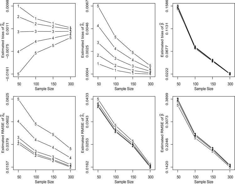
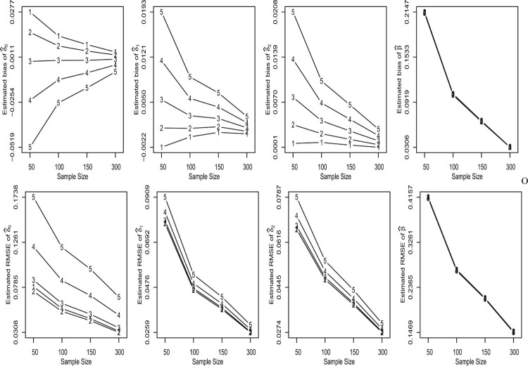
The results of the simulation experiments are presented in Figures 2 and 3 and Tables 1 and 2. From these figures and tables we can observe that

Figure 2.

Upper panel: estimated bias of ${\hat{\delta }}_0$, ${\hat{\delta }}_1$ and $\widehat{\mathrm{\text{β}}}$, respectively. Lower panel: estimated RMSE of ${\hat{\delta }}_0$, ${\hat{\delta }}_1$ and $\widehat{\mathrm{\text{β}}}$, respectively. (1: $\tau =0.10$, 2: $\tau =0.25$, 3: $\tau =0.50$, 4: $\tau =0.75$ and 5: $\tau =0.90$.)

Figure 3.

Upper panel: estimated bias of ${\hat{\delta }}_0$, ${\hat{\delta }}_1$, ${\hat{\delta }}_2$ and $\widehat{\mathrm{\text{β}}}$, respectively. Lower panel: estimated RMSE of ${\hat{\delta }}_0$, ${\hat{\delta }}_1$, ${\hat{\delta }}_2$ and $\widehat{\mathrm{\text{β}}}$, respectively. (1: $\tau =0.10$, 2: $\tau =0.25$, 3: $\tau =0.50$, 4: $\tau =0.75$ and 5: $\tau =0.90$.)

Table 1. Estimated coverage probability for ${\delta }_0$, ${\delta }_1$ and β.

	n = 50			n = 100
τ	${\delta }_0$	${\delta }_1$	β	${\delta }_0$	${\delta }_1$	β
0.10	92.86	93.97	94.52	93.89	94.24	94.95
0.25	93.85	93.77	94.54	94.32	94.25	94.96
0.50	94.21	93.49	94.65	94.62	94.17	94.84
0.75	93.65	93.19	94.41	94.41	94.21	94.81
0.90	92.83	93.04	94.19	94.03	93.85	94.58
	n = 150			n = 300
τ	${\delta }_0$	${\delta }_1$	β	${\delta }_0$	${\delta }_1$	β
0.10	94.39	94.75	94.72	94.72	94.97	94.66
0.25	94.58	94.60	94.65	95.10	94.91	94.71
0.59	94.91	94.28	94.58	95.09	94.90	94.79
0.75	94.39	94.32	94.55	94.91	95.21	94.65
0.90	94.24	94.26	94.39	94.68	95.00	94.68

Table 2. Estimated coverage probability for ${\delta }_0$, ${\delta }_1$, ${\delta }_2$ and β.

	n = 50				n = 100
τ	${\delta }_0$	${\delta }_1$	${\delta }_2$	β	${\delta }_0$	${\delta }_1$	${\delta }_2$	β
0.10	90.67	92.58	92.81	93.75	93.08	94.06	94.04	94.42
0.25	92.46	92.73	92.77	93.76	93.97	94.00	94.13	94.42
0.50	93.46	92.86	92.67	93.68	94.19	94.12	94.13	94.39
0.75	92.88	92.76	92.41	93.63	93.81	93.70	93.90	94.23
0.90	92.22	92.56	92.37	93.58	93.46	93.42	93.87	94.25
	n = 150				n = 300
τ	${\delta }_0$	${\delta }_1$	${\delta }_2$	β	${\delta }_0$	${\delta }_1$	${\delta }_2$	β
0.10	93.82	94.27	94.28	94.60	94.15	94.93	94.83	94.85
0.25	94.14	94.22	94.31	94.55	94.54	94.91	94.81	94.82
0.50	94.37	94.42	94.34	94.59	94.99	94.75	95.11	94.84
0.75	94.21	94.30	94.29	94.48	94.83	94.75	95.14	94.85
0.90	94.04	94.18	94.31	94.45	94.64	94.65	95.16	94.85

1. the highest biases and RMSE of the estimates are presented in the tails of the distribution, i.e. when $\tau =0.1\mathrm{a}\mathrm{n}\mathrm{d}0.9$;

2. the bias and RMSE of the estimates decrease as the sample size increases;

3. the estimate of β has a high bias for small sample size;

4. the coverage probability of the 95% pointwise confidence intervals of the parameters are quite close to the nominal level.

5. Applications

In this section, three real applications were presented in order to show the potentiality of the proposed regression model. For comparison purpose, in addition to the UW quantile regression model, we also considered two alternative regression models commonly used in the analysis of limited data.

In what follows the p.d.f. of the alternative regression models is presented.

• The Beta regression model introduced by Cepeda-Cuervo [7] and Ferrari and Cribari-Neto [14] has p.d.f. given by

  $$f(y\mid \mu ,\mathrm{\text{β}})=\frac{\mathrm{\Gamma }\left(\mathrm{\text{β}}\right)}{\mathrm{\Gamma }\left(\mu \mathrm{\text{β}}\right)\mathrm{\Gamma }\left(\right(1-\mu \left)\mathrm{\text{β}}\right)}{y}^{\mu \mathrm{\text{β}}-1}(1-y{)}^{(1-\mu )\mathrm{\text{β}}-1},0<y<1,$$

  where $0<\mu <1$ denotes the mean and $\mathrm{\text{β}}>0$ can be interpreted as a precision parameter.
• The Kumaraswamy regression model introduced by Mitnik and Baek [37] has p.d.f. given by

  $$f(y\mid \mu ,\mathrm{\text{β}})=\frac{\mathrm{\text{β}}\log (1-0.5)}{\log (1-{\mu }^{\mathrm{\text{β}}})}{y}^{\mathrm{\text{β}}-1}(1-y^{\mathrm{\text{β}}}{)}^{\log (1-0.5)/\log (1-{\mu }^{\mathrm{\text{β}}})-1},0<y<1,$$

  where $0<\mu <1$ denotes the median and $\mathrm{\text{β}}>0$ is the shape parameter.

To discriminate and choose the best among the proposed models, the Akaike (AIC) [1], Schwarz (BIC) [46] and Hannan–Quinn (HQIC) [22] information criteria were used. These measures are defined as follows:

$$\mathrm{A}\mathrm{I}\mathrm{C}=2p-2\log \hat{L},\mathrm{B}\mathrm{I}\mathrm{C}=\log \left(n\right)p-2\log \hat{L},\mathrm{H}\mathrm{Q}\mathrm{I}\mathrm{C}=2p\log \left(\log n\right)-2\log \hat{L},$$

where $\hat{L}$ is the likelihood evaluated at the MLE, p is the number of parameters in the model and n is the number of observations. The decision rule, in all these criteria, is favorable to the model with the lowest value [23]. In order to quantify the uncertainty associated with these criteria, the non-parametric Bootstrap approach was used to decide on the final model. We considered 10,000 independent runs and calculated the percentage of times each model was selected.

In addition, a formal test based on the Vuong likelihood ratio test for non-nested models [52] was employed to assess whether there is any significant difference in the fit of the two alternative models to unit-Weibull. The Vuong statistic to compare two regression models is defined as

$$T_{LR,NN}=\frac{1}{{\hat{\omega }}^2\sqrt{n}}\sum _{i=1}^n\log \frac{f(y_i\mid {\mathit{x}}_i,\stackrel{\mathbf{ˆ}}{\mathit{\theta }})}{g(y_i\mid {\mathit{x}}_i,\stackrel{\mathbf{ˆ}}{\mathit{\gamma }})},$$

where

$${\hat{\omega }}^2=\frac{1}{n}\sum _{i=1}^n{\left(\log \frac{f(y_i\mid {\mathit{x}}_i,\stackrel{\mathbf{ˆ}}{\mathit{\theta }})}{g(y_i\mid {\mathit{x}}_i,\stackrel{\mathbf{ˆ}}{\mathit{\gamma }})}\right)}^2-{\left[\frac{1}{n}\sum _{i=1}^n\left(\log \frac{f(y_i\mid {\mathit{x}}_i,\stackrel{\mathbf{ˆ}}{\mathit{\theta }})}{g(y_i\mid {\mathit{x}}_i,\stackrel{\mathbf{ˆ}}{\mathit{\gamma }})}\right)\right]}^2$$

is an estimator for the variance of $\left(1/\sqrt{n}\right)\sum _{i=1}^n\log \left(f(y_i\mid {\mathit{x}}_i,\stackrel{\mathbf{ˆ}}{\mathit{\theta }})/g(y_i\mid {\mathit{x}}_i,\stackrel{\mathbf{ˆ}}{\mathit{\gamma }})\right)$, $f(y_i\mid {\mathit{x}}_i,\stackrel{\mathbf{ˆ}}{\mathit{\theta }})$ and $g(y_i\mid {\mathit{x}}_i,\stackrel{\mathbf{ˆ}}{\mathit{\gamma }})$ are the corresponding rival densities evaluated at the maximum likelihood estimates. It was demonstrated that, when $n\to \mathrm{\infty }$ then $T\stackrel{D}{\to }N(0,1)$. Therefore, at a significance level of $\alpha \mathrm{\%}$ distribution equivalence is rejected if $|T|<z_{\alpha /2}$.

Finally, the maximum likelihood estimates were obtained using the dual quasi-Newton algorithm available in the SAS/NLMIXED procedure [44]. The asymptotic standard errors and confidence intervals were computed using the inverse of the observed Fisher information matrix. The SAS codes are available upon request.

5.1. Recovery rate of CD34+ cells data

In this application, the data correspond to a study conducted with 239 patient between 2003 and 2008 at the Edmonton Hematopoietic Stem Cell Lab in Cross Cancer Institute – Alberta Health Services. The data set was extracted from [55] and the goal is to model the recovery rate of CD34+ cells after peripheral blood stem cell (PBSC) transplants. The covariates associated with this response variable are

• $x_1$ (Gender): 0 for female, 1 for male;

• $x_2$ (Chemotherapy): 0 for receiving chemotherapy on a one-day protocol, 1 for a 3-day protocol;

• $x_3$ (Age): adjusted patient's age, i.e. the current age minus 40.

The regression structure assumed for ${\mu }_i$ is given by

$$\mathrm{l}\mathrm{o}\mathrm{g}\mathrm{i}\mathrm{t}\left({\mu }_i\right)={\delta }_0+{\delta }_1{x}_{i1}+{\delta }_2{x}_{i2}+{\delta }_3{x}_{i3},i=1,\dots ,239,$$ (14)

where ${\mu }_i$ denotes the median in the unit-Weibull and Kumaraswamy models, whereas in the Beta model ${\mu }_i$ denotes the mean.

Table 3 gives the maximum likelihood parameter estimates and the 95% pointwise confidence intervals for all the rival models.

Table 3. The maximum likelihood parameter estimates and the 95% pointwise confidence intervals – recovery rate of CD34+ cells data.

	unit-Weibull		Kumaraswamy		Beta
Parameter	MLE	95% C.I.	MLE	95% C.I.	MLE	95% C.I.
${\delta }_0$	0.9619	(0.7031, 1.2208)	1.1997	(0.9259, 1.4736)	0.9990	(0.7460, 1.2521)
${\delta }_1$	0.0174	(0.0075, 0.0273)	0.0107	(−0.0008, 0.0223)	0.0142	(0.0037, 0.0247)
${\delta }_2$	0.2816	(0.0887, 0.4744)	0.1833	(−0.0421, 0.4088)	0.2116	(0.0083, 0.4150)
${\delta }_3$	0.1033	(−0.0816, 0.2883)	0.0418	(−0.1454, 0.2290)	0.0659	(−0.1182, 0.2500)
β	1.6802	(1.5174, 1.8430)	6.7274	(5.8371, 7.6178)	11.3447	(9.3494, 13.3401)

In Table 4 the comparison of the fit of the three proposed models is presented through the values of the statistics used as selection criteria. The three information criteria evaluated indicate that the unit-Weibull regression model presented a better fit when compared to the competing models for the recovery rate of CD34+ data. This conclusion is reinforced by the percentage of times that each model was selected. Considering a level of $5\mathrm{\%}$ of significance, the results of the Vuong test indicate that there is insufficient sample evidence that the Beta and unit-Weibull models differ significantly, and the unit-Weibull fit was shown superior to all the others.

Table 4. The likelihood-based statistics of fit – recovery rate of CD34+ cells data.

Criteria	unit-Weibull	Kumaraswamy	Beta
AIC (%)${}^{\mathrm{a}}$	−388.0932 (44.47%)	−375.6599 (23.87%)	−381.7912 (31.56%)
BIC (% )	−370.7109 (44.56%)	−358.2775 (23.86%)	−364.4089 (31.58%)
HQIC (%)	−381.0886 (44.49%)	−368.6553 (23.90%)	−374.7866 (31.61%)
Voung	–	1.7117	1.0590
(p-value)		(0.0435)	(0.1448)

${}^{\mathrm{a}}$ % of times out of 10,000 non-parametric Bootstrap runs that the model is selected.

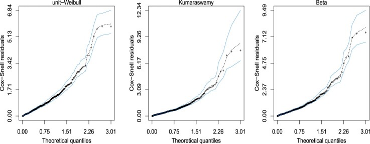
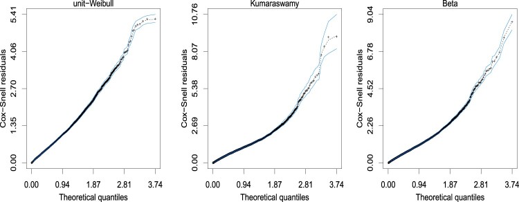
In order to assess if the model is appropriate, in Figure 4 it is shown the half-normal plots with simulated envelopes for the Cox–Snell residuals. Figure 4 indicates a good fit of the unit-Weibull regression model to the recovery rate of CD34+ cells data.

Figure 4.

The half-normal plot with simulated envelope for the Cox–Snell residuals – recovery rate of CD34+ cells data.

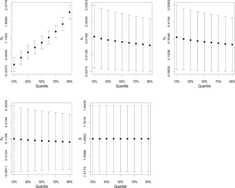
The impact of different τ's on the estimates of β and ${\delta }_i$, $i=0,\dots ,3$, is illustrated in Figure 5.

Figure 5.

The parameter estimates and the 95% pointwise confidence intervals for the UW model and $\tau =0.1,0.2,\dots ,0.8\mathrm{a}\mathrm{n}\mathrm{d}0.9$ – recovery rate of CD34+ cells data.

5.2. Access to piped water supply data

In this application, we consider the data set related to the access of people in households with piped water supply in the cities of Brazil from the Southeast and Northeast regions. We are interested in analyzing the association between proportion of households with piped water supply and some socio-demographic variables of these cities. The data are available from http://atlasbrasil.org.br/2013/ and represent 3457 cities during the census in 2010. The response variable y (Phpws) is the proportion of households with piped water supply. The covariates associated with this response variable are

• $x_1$ (HDI): human development index;

• $x_2$ (Region): 0 for Southeast, 1 for Northeast;

• $x_3$ (Incpc): income per capita;

• $x_4$ (Pop): total population.

The regression structure assumed for ${\mu }_i$ is given by

$$\mathrm{l}\mathrm{o}\mathrm{g}\mathrm{i}\mathrm{t}\left({\mu }_i\right)={\delta }_0+{\delta }_1{x}_{i1}+{\delta }_2{x}_{i2}+{\delta }_3{x}_{i3}+{\delta }_4\log \left(x_{i4}\right),i=1,\dots ,3457.$$ (15)

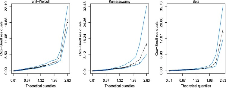
The point estimates and the 95% pointwise confidence intervals for the parameters of the considered three regression models are given in Table 5. Table 6 gives the values of the likelihood-based statistics and the Vuong test of equivalence of the considered models. This table shows that the unit-Weibull regression model provides the best fit, since it has the lowest values of AIC, BIC and HQIC statistics. Moreover, the Vuong test shows that the unit-Weibull regression model is not equivalent to either the Kumaraswamy or the Beta regression models. These conclusions are also supported by the half-normal plots for the Cox–Snell residuals with simulated envelopes exhibited in Figure 6.

Table 5. The maximum likelihood parameter estimates and the 95% pointwise confidence intervals – access to piped water supply data.

	unit-Weibull		Kumaraswamy		Beta
Parameter	MLE	95% C.I.	MLE	95% C.I.	MLE	95% C.I.
${\delta }_0$	−6.5145	(−7.1556, −5.8733)	−1.6259	(−2.2572, −0.9947)	−3.8943	(−4.4598, −3.3289)
${\delta }_1$	11.8262	(10.7368, 12.9155)	4.8432	(3.6989, 5.9874)	8.3186	(7.3339, 9.3034)
${\delta }_2$	−0.2699	(−0.3668, −0.1730)	−0.0786	(−0.1815, 0.0243)	−0.1940	(−0.2774, −0.1106)
${\delta }_3$	0.0003	(−0.0001, 0.0006)	0.0021	(0.0016, 0.0026)	0.0005	(0.0001, 0.0008)
${\delta }_4$	0.1055	(0.0751, 0.1358)	−0.0473	(−0.0803, −0.0143)	0.0157	(−0.0122, 0.0436)
β	1.1883	(1.1604, 1.2161)	5.7996	(5.5631, 6.0360)	9.5884	(9.1243, 10.0525)

Table 6. The likelihood-based statistics – access to piped water supply.

Criteria	unit-Weibull	Kumaraswamy	Beta
AIC (%)${}^{\mathrm{a}}$	−7982.0762 (90.78%)	−7176.4979 (0.00%)	−7660.1747 (9.22%)
BIC (%)	−7945.1872 (90.78%)	−7139.6089 (0.00%)	−7623.2858 (9.22%)
HQIC (%)	−7968.9027 (90.72%)	−7163.3244 (0.00%)	−7647.0012 (9.28%)
Vuong	–	7.2248	3.0340
(p-value)		(0.0000)	(0.0012)

${}^{\mathrm{a}}$ % of times out of 10,000 non-parametric Bootstrap runs that the model is selected.

Figure 6.

The half-normal plot with simulated envelope for the Cox–Snell residuals – access to piped water supply data.

The results obtained from the unit-Weibull regression model indicate that only the covariate $x_3$ (Incpc) is not statistically significant to explain the response variable, since the confidence interval for ${\delta }_3$ includes the zero value. It is also noted that there is a positive relationship between the median response (proportion of households with piped water supply) and the human development index of the city and the logarithm of the total population. This means that cities with greater values of HDI and/or total population tend to have more proportion of households with piped water supply. On the other hand, it was observed that the cities localized in the Northeast region have less proportion of households with piped water supply than the cities in the Southeast. It is natural to expect that the shape parameter (β) will not be influenced by the percentile unless it is dependent on the covariates.

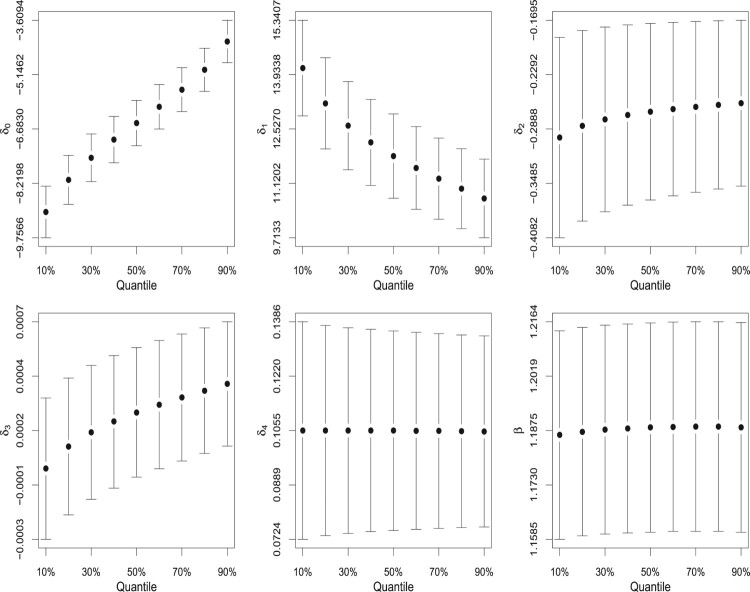
Figure 7 displays the maximum likelihood estimates and the 95% pointwise confidence interval for the parameters of the UW regression model considering different values for the quantiles. It is observed that the quantile regression could be more interesting than the conditional mean regression because it allows a complete view of the condition distribution by studying the effect of explanatory variables on the response in distinct quantiles. For instance, a close inspection in Figure 7 reveals that as τ increases the estimates of ${\delta }_1$ become smaller, indicating that the human development is more important to explain smaller quantiles of the response variable.

Figure 7.

Parameter estimates and its 95% pointwise confidence intervals for the UW model considering $\tau =0.1,0.2,\dots ,0.9$ – access to piped water supply.

5.3. Risk management cost effectiveness data

The data set considered is presented by Schmit and Roth [45], and corresponds to the 73 responses to a questionnaire sent to 374 risk managers of large North American organizations. The objective of Schmit and Roth [45] was to evaluate the cost effectiveness with the management philosophy of controlling the company's exposure to various property losses and accidents, taking into account company characteristics such as size and type of industry.

The response variable y (Firm cost) is the firm-specific ratio of premiums plus uninsured losses divided by total assets. The covariates associated with this response variable are

• $x_1$ (Assume): firm-specific ratio of the summation of per occurrence retention levels, as measured by the corporate risk manager;

• $x_2$ (Cap): 1 if the firm uses a captive and 0 otherwise;

• $x_3$ (Sizelog): log of the firm's total asset value;

• $x_4$ (Indcost): industry average of premiums plus uninsured losses divided by total assets, as measured by the 1985 Cost of Risk Survey (a measure of risk);

• $x_5$ (Central): importance of local manager in choosing local retention levels, as measured by the corporate risk manager;

• $x_6$ (Soph): importance of analytical tools in making risk management decisions, as measured by the corporate risk manager.

The regression structure assumed for ${\mu }_i$ is given by

$$\mathrm{l}\mathrm{o}\mathrm{g}\mathrm{i}\mathrm{t}\left({\mu }_i\right)={\delta }_0+{\delta }_1{x}_{i1}+{\delta }_2{x}_{i2}+{\delta }_3{x}_{i3}+{\delta }_4{x}_{i4}+{\delta }_5{x}_{i5}+{\delta }_6{x}_{i6},i=1,\dots ,73.$$ (16)

The point estimates and the $95\mathrm{\%}$ pointwise confidence intervals for the parameters of the considered three regression models are given in Table 7. Table 8 gives the values of the likelihood-based statistics and the Vuong test of equivalence of the considered models. This table shows that the unit-Weibull regression model provide the best fit, since it has the lowest values of AIC, BIC and HQIC statistics. Moreover, the Vuong test shows that the unit-Weibull regression model is not equivalent to either the Kumaraswamy or the Beta regression models. These conclusions are also supported by the half-normal plots for the Cox–Snell residuals with simulated envelopes shown in Figure 8.

Table 7. The maximum likelihood parameter estimates and the 95% pointwise confidence intervals – risk management cost effectiveness data.

	unit-Weibull		Kumaraswamy		Beta
Parameter	MLE	95% C.I.	MLE	95% C.I.	MLE	95% C.I.
${\delta }_0$	3.4712	(1.2889, 5.6535)	2.5387	(−0.4998, 5.5773)	1.8880	(−0.4096, 4.1855)
${\delta }_1$	−0.0076	(−0.0332, 0.0179)	−0.0364	(−0.0709, −0.0019)	−0.0121	(−0.0394, 0.0151)
${\delta }_2$	0.1278	(−0.3635, 0.6190)	0.5964	(−0.1686, 1.3615)	0.1780	(−0.2763, 0.6322)
${\delta }_3$	−0.8043	(−1.0451, −0.5635)	−0.7981	(−1.1143, −0.4820)	−0.5115	(−0.7524, −0.2705)
${\delta }_4$	1.4394	(0.6353, 2.2435)	5.2568	(2.4429, 8.0707)	1.2362	(0.3359, 2.1366)
${\delta }_5$	−0.0241	(−0.1913, 0.1430)	−0.0278	(−0.2621, 0.2065)	−0.0122	(−0.1836, 0.1593)
${\delta }_6$	−0.0023	(−0.0454, 0.0408)	−0.0274	(−0.0902, 0.0354)	−0.0037	(−0.0455, 0.0380)
β	3.3533	(2.7278, 3.9787)	0.9784	(0.7709, 1.1860)	6.3305	(4.1300, 8.5311)

Table 8. The likelihood-based statistics of fit – risk management cost effectiveness data.

Criteria	unit-Weibull	Kumaraswamy	Beta
AIC (%)${}^{\mathrm{a}}$	−206.2227 (47.33%)	−181.6534 (34.22%)	−159.4460 (18.45%)
BIC (%)	−187.8990 (47.34%)	−163.3297 (34.22%)	−141.1223 (18.44%)
HQIC (%)	−198.9204 (47.32%)	−174.3511 (34.23%)	−152.1437 (18.45%)
Vuong	–	2.1513	4.5817
(p-value)		(0.0157)	(0.0000)

${}^{\mathrm{a}}$ % of times out of 10,000 non-parametric Bootstrap runs that the model is selected.

Figure 8.

The half-normal plot with simulated envelope for the Cox–Snell residuals – risk management cost effectiveness data.

From the inference results obtained for the UW regression model it can be inferred that the covariates $x_3$ (Size) and $x_4$ (Indcost) are statistically significant at the usual nominal levels. Additionally, it is noteworthy that there is a negative relationship between the median response, that is, the measure of the firm's risk management cost effectiveness, and the log of the firm's total asset value. On the other hand, the measure of risk (Indcost) has a positive impact on the median response.

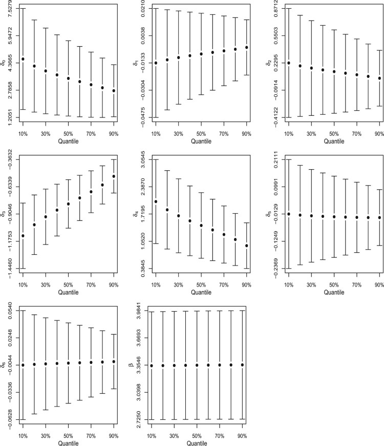
Finally, we present in Figure 9 the parameter estimates and its 95% confidence interval of the UW regression model assuming different values for the quantiles. It can be seen that as τ increases the coefficient of firm's total asset value (${\delta }_3$) becomes bigger. In contrast, for the Indcost covariate it is observed that as τ increases the estimates of ${\delta }_4$ becomes smaller.

Figure 9.

Parameter estimates and its 95% pointwise confidence intervals for the UW model considering $\tau =0.1,0.2,\dots ,0.9$ – risk management cost effectiveness data.

As a final comment on the applications, we can observe that the estimates of the median regression coefficients are clearly affected by the choice of the distribution of the response variable, unit-Weibull or Kumaraswamy. As pointed out by a reviewer, in application 2 one estimated coefficient, ${\delta }_4$, change of sign and the confidence intervals do not overlap. In the unit-Weibull distribution, we have a positive effect of $\log \left(x_4\right)$ on the median of the response variable distribution while this effect is negative if the Kumaraswamy distribution is adopted. This fact emphasizes the need to consider different distributions in the analysis of real data and to decide on the distribution with better goodness of fit. As mentioned in [42]

Goodness of fit is concerned with assessing the validity of models involving statistical distributions, an essential and sometimes forgotten aspect of the modeling exercise. One can only speculate on how many wrong decisions are made due to the use of an incorrect model

In our applications, we have strong evidence that the proposed distribution is more appropriate. With respect to signal change in application 2, the percentage of times that the Kumaraswamy distribution was chosen in 10,000 replications was equal to zero. From the same simulation study, for the unit-Weibull and Kumaraswamy distribution, we observed only 1 out of 10,000 change in the sign of coefficient associated to $\log \left(x_4\right)$.

6. Conclusions

As pointed out by Noufaily [40] and Noufaily and Jones [39], most of the literature concerning quantile regression models has involved non-parametric components either in the functional form of the regression equation or the distribution of the random component (or both). In this context, parametric distributions for the response variable were rarely used. To explore a fully parametric approach for quantile regression, these authors have considered the Generalized Gamma distribution for the response variable. For a variable on the unit interval, Mitnik and Baek [37] and Bayes et al. [5] have considered the Kumaraswamy distribution. In the paper herein, the unit-Weibull distribution was considered as an alternative to the Kumaraswamy distribution. For this purpose, the proposed model was reparameterized in terms of its quantiles. A Monte Carlo simulation study was performed and has shown that the parameters were well estimated in terms of the bias and mean-squared error of their respective estimators. Three real datasets were analyzed for illustrative and model comparison purposes. For these datasets, the unit-Weibull quantile regression model has outperformed the Kumaraswamy and Beta models according to three information criteria and the half-normal plots for the Cox–Snell residuals. Although the presented formulation looks like a simple algebraic exercise, the proposed model has proved to be useful, simple to implement and that can be straightforwardly extended to accommodate observations existing at zero, one or both.

Funding Statement

Josmar Mazucheli gratefully acknowledge the partial financial support from Fundação Araucária (grant 064/2019 – UEM/Fundação Araucária).

Disclosure statement

No potential conflict of interest was reported by the authors.

ORCID

J. Mazucheli http://orcid.org/0000-0001-6740-0445

R. P. de Oliveira http://orcid.org/0000-0001-6134-5975

References

- 1.Akaike H., A new look at the statistical model identification, 19 (1974), pp. 716–723. [Google Scholar]
- 2.Atkinson A.C., Two graphical displays for outlying and influential observations in regression, Biometrika 68 (1981), pp. 13–20. doi: 10.1093/biomet/68.1.13 [DOI] [Google Scholar]
- 3.Atkinson A.C., Plots, Transformations, and Regression: An Introduction to Graphical Methods of Diagnostic Regression Analysis, Oxford University Press, New York, 1985. [Google Scholar]
- 4.Barndorff-Nielsen O. and Jørgensen B., Some parametric models on the Simplex, J. Multivar. Anal. 39 (1991), pp. 106–116. doi: 10.1016/0047-259X(91)90008-P [DOI] [Google Scholar]
- 5.Bayes C.L., Bazán J.L., and de Castro M., A quantile parametric mixed regression model for bounded response variables, Stat. Interface 10 (2017), pp. 483–493. doi: 10.4310/SII.2017.v10.n3.a11 [DOI] [Google Scholar]
- 6.Bayes C.L., Bazán J.L., and García C., A new robust regression model for proportions, Bayesian Anal. 7 (2012), pp. 841–866. doi: 10.1214/12-BA728 [DOI] [Google Scholar]
- 7.Cepeda-Cuervo E., Variability modeling in generalized linear models, Ph.D. diss., Mathematics Institute, Universidade Federal do Rio de Janeiro, 2001.
- 8.Collet D., Modelling Binary Data, 2nd ed., Chapman & Hall/CRC, New York, 2003. [Google Scholar]
- 9.Cook D.O., Kieschnick R., and McCullough B.D., Regression analysis of proportions in finance with self selection, J. Empir. Financ. 15 (2008), pp. 860–867. doi: 10.1016/j.jempfin.2008.02.001 [DOI] [Google Scholar]
- 10.Cox D.R. and Snell E.J., A general definition of residuals, J. R. Stat. Soc. Ser. B 30 (1968), pp. 248–275. [Google Scholar]
- 11.Cribari-Neto F. and Souza T.C., Religious belief and intelligence: Worldwide evidence, Intelligence 41 (2013), pp. 482–489. doi: 10.1016/j.intell.2013.06.011 [DOI] [Google Scholar]
- 12.Cribari-Neto F. and Zeileis A., Beta regression in R, J. Stat. Softw. 34 (2010), pp. 1–24. doi: 10.18637/jss.v034.i02 [DOI] [Google Scholar]
- 13.da Paz R.F., Alternative regression models to beta distribution under Bayesian approach, Ph.D. diss., Instituto de Ciências Matemáticas e de Computaç ao, Universidade de S ao Paulo, S ao Carlos, Brazil, 2017.
- 14.Ferrari S. and Cribari-Neto F., Beta regression for modelling rates and proportions, J. Appl. Stat. 31 (2004), pp. 799–815. doi: 10.1080/0266476042000214501 [DOI] [Google Scholar]
- 15.Geraci M., Qtools: A collection of models and tools for quantile inference, R J. 8 (2016), pp. 117–138. doi: 10.32614/RJ-2016-037 [DOI] [Google Scholar]
- 16.Geraci M. and Jones M.C., Improved transformation-based quantile regression, Can. J. Stat. 43 (2015), pp. 118–132. doi: 10.1002/cjs.11240 [DOI] [Google Scholar]
- 17.Gómez-Déniz E., Sordo M.A., and Calderín-Ojeda E., The log-Lindley distribution as an alternative to the beta regression model with applications in insurance, Insur.: Math. Econ. 54 (2014), pp. 49–57. [Google Scholar]
- 18.Grassia A., On a family of distributions with argument between 0 and 1 obtained by transformation of the Gamma distribution and derived compound distributions, Aust. J. Stat. 19 (1977), pp. 108–114. doi: 10.1111/j.1467-842X.1977.tb01277.x [DOI] [Google Scholar]
- 19.Gupta R. and Kundu D., Generalized exponential distributions, Aust. N. Z. J. Stat. 58 (1999), pp. 173–188. doi: 10.1111/1467-842X.00072 [DOI] [Google Scholar]
- 20.Gupta A.K. and Nadarajah S. (eds.), Handbook of Beta Distribution and Its Applications, Marcel Dekker, New York, 2004. [Google Scholar]
- 21.Hahn E.D., Mixture densities for project management activity times: A robust approach to PERT, Eur. J. Oper. Res. 188 (2008), pp. 450–459. doi: 10.1016/j.ejor.2007.04.032 [DOI] [Google Scholar]
- 22.Hannan E.J. and Quinn B.G., The determination of the order of an autoregression, J. R. Stat. Soc.: Ser. B (Methodol.) 41 (1979), pp. 190–195. [Google Scholar]
- 23.Held L. and Sabanés Bové D., Applied Statistical Inference – Likelihood and Bayes, Springer, New York, 2014. [Google Scholar]
- 24.Hunger M., Baumert J., and Holle R., Analysis of SF-6D index data: Is beta regression appropriate?, Value Health 14 (2011), pp. 759–767. doi: 10.1016/j.jval.2010.12.009 [DOI] [PubMed] [Google Scholar]
- 25.Johnson N.L., Systems of frequency curves generated by methods of translation, Biometrika 36 (1949), pp. 149–176. doi: 10.1093/biomet/36.1-2.149 [DOI] [PubMed] [Google Scholar]
- 26.Kieschnick R. and McCullough B.D., Regression analysis of variates observed on (0, 1): Percentages, proportions and fractions, Stat. Modelling 3 (2003), pp. 193–213. doi: 10.1191/1471082X03st053oa [DOI] [Google Scholar]
- 27.Koenker R. and Bassett G., Regression quantiles, Econometrica 46 (1978), pp. 33–50. doi: 10.2307/1913643 [DOI] [Google Scholar]
- 28.Kumaraswamy P., A generalized probability density function for double-bounded random processes, J. Hydrol. (Amst) 46 (1980), pp. 79–88. doi: 10.1016/0022-1694(80)90036-0 [DOI] [Google Scholar]
- 29.Kutner M.H., Nachtsheim C.J., Neter J., and Li W., Applied Linear Statistical Models, 5th ed., McGraw-HillfIrwin, New York, 2005. [Google Scholar]
- 30.Lawless J.F., Statistical Models and Methods for Lifetime Data, 2nd ed., John Wiley and Sons, New York, 2003. [Google Scholar]
- 31.Lee E.T. and Wang J.W., Statistical Methods for Survival Data Analysis, 3rd ed., Wiley Series in Probability and Statistics, Hoboken, NJ, 2003. [Google Scholar]
- 32.Lehmann E.L. and Casella G., Theory of Point Estimation, 2nd ed., Springer Verlag, New York, 1998. [Google Scholar]
- 33.Lemonte A.J. and Bazán J.L., New class of Johnson distributions and its associated regression model for rates and proportions, Biometrical J. 58 (2015), pp. 727–746. doi: 10.1002/bimj.201500030 [DOI] [PubMed] [Google Scholar]
- 34.Lindsay B.G. and Li B., On second-order optimality of the observed Fisher information, Ann. Stat. 25 (1997), pp. 2172–2199. doi: 10.1214/aos/1069362393 [DOI] [Google Scholar]
- 35.Mazucheli J., Menezes A.F.B., and Chakraborty S., On the one parameter unit-Lindley distribution and its associated regression model for proportion data, arXiv:1801.02512v1 (2018).
- 36.Mazucheli J., Menezes A.F.B., and Ghitany M.E., The unit-Weibull distribution and associated inference, J. Appl. Probab. Stat. 13 (2018), pp. 1–22. [Google Scholar]
- 37.Mitnik P.A. and Baek S., The Kumaraswamy distribution: Median-dispersion re-parameterizations for regression modeling and simulation-based estimation, Stat. Pap. 54 (2013), pp. 177–192. doi: 10.1007/s00362-011-0417-y [DOI] [Google Scholar]
- 38.Mousa A.M., El-Sheikh A.A., and Abdel-Fattah M.A., A gamma regression for bounded continuous variables, Adv. Appl. Stat. 49 (2016), pp. 305. [Google Scholar]
- 39.Noufaily A. and Jones M.C., Parametric quantile regression based on the generalized gamma distribution, J. R. Stat. Soc.: Ser. C (Appl. Stat.) 62 (2013), pp. 723–740. [Google Scholar]
- 40.Noufaily A., Parametric quantile regression based on the generalised gamma distribution, Ph.D. diss., Department of Mathematics and Statistics, The Open University, Milton Keynes, 2011.
- 41.Papke L.E. and Wooldridge J.M., Econometric methods for fractional response variables with an application to 401(k) plan participation rates, J. Appl. Economet. 11 (1996), pp. 619–632. doi: [DOI] [Google Scholar]
- 42.Rayner J.C.W., Thas O., and Best D.J., Smooth Tests of Goodness of Fit: Using R, Wily Series in Probability and Statistics, John Wily & Songs (Asia), Singapore, Chichester, 2009.
- 43.Santos B. and Bolfarine H., Bayesian analysis for zero-or-one inflated proportion data using quantile regression, J. Stat. Comput. Simul. 85 (2015), pp. 3579–3593. doi: 10.1080/00949655.2014.986733 [DOI] [Google Scholar]
- 44.SAS , The NLMIXED Procedure, SAS/STAT® User's Guide, Version 9.4, Cary, NC: SAS Institute Inc., 2010.
- 45.Schmit J.T. and Roth K., Cost effectiveness of risk management practices, J. Risk Insur. 57 (1990), pp. 455–470. doi: 10.2307/252842 [DOI] [Google Scholar]
- 46.Schwarz G. et al., Estimating the dimension of a model, Ann. Stat. 6 (1978), pp. 461–464. doi: 10.1214/aos/1176344136 [DOI] [Google Scholar]
- 47.Shou Y. and Smithson M., cdfquantreg: Quantile Regression for Random Variables on the Unit Interval (2018). https://CRAN.R-project.org/package=cdfquantreg, R package version 1.2.0.
- 48.Smithson M. and Shou Y., CDF-quantile distributions for modelling random variables on the unit interval, Brit. J. Math. Stat. Psychol. 70 (2017), pp. 412–438. doi: 10.1111/bmsp.12091 [DOI] [PubMed] [Google Scholar]
- 49.Souza T.C. and Cribari-Neto F., Intelligence, religiosity and homosexuality non-acceptance: Empirical evidence, Intelligence 52 (2015), pp. 63–70. doi: 10.1016/j.intell.2015.07.003 [DOI] [Google Scholar]
- 50.Tadikamalla P.R., On a family of distributions obtained by the transformation of the gamma distribution, J. Stat. Comput. Simul. 13 (1981), pp. 209–214. doi: 10.1080/00949658108810497 [DOI] [Google Scholar]
- 51.Tadikamalla P.R. and Johnson N.L., Systems of frequency curves generated by transformations of logistic variables, Biometrika 69 (1982), pp. 461–465. doi: 10.1093/biomet/69.2.461 [DOI] [Google Scholar]
- 52.Vuong Q.H., Likelihood ratio tests for model selection and non-nested hypotheses, Econometrica 57 (1989), pp. 307–333. doi: 10.2307/1912557 [DOI] [Google Scholar]
- 53.Weibull W., A statistical distribution of wide applicability, J. Appl. Mech. 18 (1951), pp. 293–297. [Google Scholar]
- 54.Yu K., Lu Z. and Stander J., Quantile regression: Applications and current research areas, J. R. Stat. Soc.: Ser. D (Stat.) 52 (2003), pp. 331–350. doi: 10.1111/1467-9884.00363 [DOI] [Google Scholar]
- 55.Zhang P., Qiu Z., and Shi C., simplexreg: An R package for regression analysis of proportional data using the simplex distribution, J. Stat. Softw. 71 (2016), pp. 1–21. [Google Scholar]