Extremal index blocks estimator: the threshold and the block size choice

Abstract

The main objective of Statistics of Extremes is the estimation of probabilities of rare events. When extending the analysis of the limiting behaviour of the extreme values from independent and identically distributed sequences to stationary sequences a key parameter appears, the extremal index θ, whose accurate estimation is not easy. Here we focus on the estimation of θ using blocks estimators, that can be constructed by using disjoint or sliding blocks. The asymptotic properties for both procedures were studied and compared but both blocks estimators require the choice of a threshold and a block length. Some criteria have appeared for the choice of those nuisance quantities but some research is still needed. We will show how the threshold and the block size choices can affect the estimates. However the main objective of this work is to revisit another estimation procedure that only depends on the block length, although some conditions on the underlying process need to be verified. The associated estimator presents nice asymptotic properties, and for finite samples is here illustrated a stability criterion for choosing the block length and then obtaining the θ estimate. A large simulation study has been performed and an application to daily mean flow discharge rate in the hydrometric station of Fragas da Torre in river Paiva, data collected from 1 October 1946 to 30 April 2012 is done.

1. Motivation and introduction

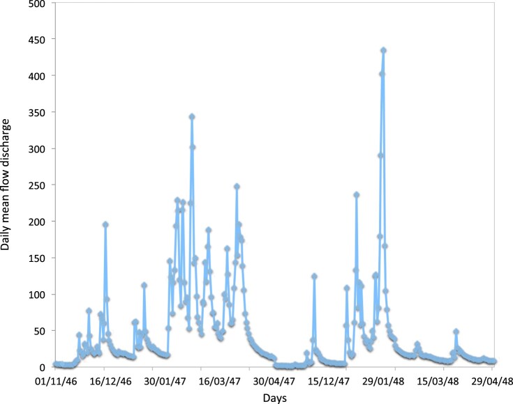
Extreme Value Theory is an area of increasingly vast applications in a very large range of environmental problems, such as burned areas (Díaz-Delgado et al. [8] and Schoenberg et al. [24]) and earthquake thermodynamics (Lavenda and Cipollone [16]), to mention a few recent applications. In many cases, another phenomenon can be observed, namely the presence of clustering of very large or very small values (extremes) of the data. Figure 1 displays the occurrence of clusters of high values in a case study of daily mean flow discharge rate values (${\mathrm{m}}^3/\mathrm{s}$) from the hydrometric station at Fragas da Torre collected from the ‘SNIRH: Sistema Nacional de Informação dos Recursos Hídricos’. A pronounced temporal clustering of the extreme values can be seen, indicating the presence of local dependence in the extremes. Therefore, quantifying the nature of the dependence structure as well as the duration of extreme events becomes an essential part of the understanding of this time series data.

Figure 1.

Daily mean flow discharge rate values (${\mathrm{m}}^3/\mathrm{s}$) from 1 November 1946 to 30 April 1947 and from 1 November 1947 to 30 April 1948 from hydrometric station at Fragas da Torre.

The extremal index (EI), usually denoted by θ, is the main parameter that describes and quantifies the clustering characteristics of the extreme values in many stationary time series. Its formal definition is given in Section 2.

This work was motivated by that real case, with the objective of studying and comparing methods to estimate the EI. Classical inference for the cluster size distribution has been mainly based in the blocks method and in the runs method, see Smith and Weissman [26] and Weissman and Novak [28]. Those procedures require that the block size and the threshold be chosen, and the estimates strongly depend on that choice. We will illustrate that dependence for some stationary processes and some finite samples generated from those processes.

In Section 2, we introduce the notations used throughout the article, the definition and some probabilistic characterizations of the EI are briefly reminded. Those characterizations gave rise to the definition of some estimators. The blocks estimator, Weissman and Novak [28], will be the classical estimator to be considered as a comparison with another blocks estimator, derived under some conditions on the stationary process and a different definition of blocks. In Section 3. the classical blocks method, properties of blocks estimators and their difficulties are discussed and illustrated through some simulated samples. The new approach for defining blocks and the conditions for the definition of a new estimator are presented in Section 4. Consistence and asymptotic distributional properties of the estimator are studied. The EI estimation under this approach is illustrated for some simulated samples. In Section 5 an heuristic procedure based on a stability criterion is considered to automatically choose the block size and to obtain the θ estimate. The real case study that motivated this study, will be considered in Section 6 and some general comments are pointed out in Section 7.

2. Extremal index: definition and characterization

In many practical applications extreme conditions often persist over several consecutive observations. Under adequate general local and asymptotic dependence conditions, the limiting point process of exceedances of a high level $u_n$ by $X_1,\dots ,X_n$, after a suitable normalization is a homogeneous compound Poisson process with intensity $\theta \tau$ and limiting cluster size distribution, π (Hsing et al. [14]). That constant θ, EI, has an important role in extreme value theory for weakly dependent processes, reflecting the effect of clustering of extremes observation on the limiting distribution of the maximum. The EI is the quantity that measures the amount of clustering of the extremes in a stationary sequence.

Definition 2.1 Leadbetter et al. [18] —

Suppose that $\{X_n{\}}_{n\ge 1}$ is a strictly stationary sequence of random variables with marginal distribution function (d.f.) F. This sequence is said to have an extremal index $\theta \in [0,1]$ if, for each $\tau >0$, there exists a sequence of levels $u_n\equiv u_n(\tau )$, such that

$$n\{1-F(u_n)\}\underset{n\to \mathrm{\infty }}{⟶}\tau \mathrm{and}\mathbb{P}\{M_{1,n}\le u_n(\tau )\}\underset{n\to \mathrm{\infty }}{⟶}\exp (-\theta \tau ),$$

where $M_{1,n}=max\{X_1,\dots ,X_n\}$.

When $\theta =1$ the exceedances of high thresholds tend to occur isolated, as in the independent context. If $\theta <1$ we have groups of exceedances in the limit.

The EI measures the relationship between the dependence structure of the data and the behavior of the exceedances over a high threshold $u_n$.

Dependence in stationary sequences can take different forms, and it is impossible to develop a general characterization of the behavior of extremes unless some constraints are imposed. It is usual to assume a condition that limits the extend of long-range dependence at extreme levels, so that the events $X_i>u$ and $X_j>u$ are approximately independent, provided that u is high enough, and time points i and j have a large separation. Let us denote $F_{i_1,i_2,\dots ,i_p}(u_1,u_2,\dots ,u_p):=\mathbb{P}(X_{i_1}\le u_1,X_{i_2}\le u_2,\dots ,X_{i_p}\le u_p)$, the joint d.f. of $(X_{i_1},X_{i_2},\dots ,X_{i_p})$ for any arbitrary positive integers $(i_1,i_2,\dots ,i_p)$.

Definition 2.2 $D(u_n)$ condition (Leadbetter et al. [18]) —

The $D(u_n)$ condition holds for a stationary sequence if for every integers p, q and $i_1<i_2<\cdots <i_p<j_i<j_2<\cdots <j_q<n$ such that $j_1-i_p>\ell \equiv {\ell }_n$, we have

$$\begin{array}{rl}& |F_{i_1,i_2,\dots ,i_p,j_1,j_2,\dots ,j_q}(u_n,u_n,\dots ,u_n)\\ & -F_{i_1,i_2,\dots ,i_p}(u_n,u_n,\dots ,u_n)F_{j_1{j}_2,\dots ,j_q}(u_n,u_n,\dots ,u_n)|\le {\alpha }_{n,\ell },\end{array}$$

where $\underset{n\to \mathrm{\infty }}{lim}{\alpha }_{n,{\ell }_n}=0$ for some sequence $\{{\ell }_n=o(n)\}$.

Let $\{X_n{\}}_{n\ge 1}$ be a strictly stationary sequence of random variables that satisfies the $D(u_n)$ condition of Leadbetter et al. [18] and has a marginal distribution function F. For large n and $u_n$,

$$\mathbb{P}\{M_{1,n}\le u_n\}\approx F^{n\theta }(u_n).$$

Further, if there exist normalizing constants $a_n\in {\mathbb{R}}^{+}$ and $b_n\in \mathbb{R}$ such that $F^n(a_{n}x+b_n)\underset{n\to \mathrm{\infty }}{⟶}G(x),$ then $G(x)$ is the distribution function of a GEV distribution, and

$$\mathbb{P}\{M_{1,n}\le u_n\}\underset{n\to \mathrm{\infty }}{⟶}H(x)=G^{\theta }(x).$$

The corresponding result for $M_{1,n}^{\ast }=max\{X_1^{\ast },\dots ,X_n^{\ast }\}$ where $X_1^{\ast },X_2^{\ast },\dots$ are independent variables with distribution function F, gives the limiting distribution function $G(x)=H(x{)}^{1/\theta }$. Hence, the EI is a key parameter for the distribution of sample extremes.

For illustration of the behaviour of a stationary process compared with the correspondent i.i.d. sequence and the effect let us consider the following example:

Example 2.3 A Moving Maximum Process, (Süveges [27]) —

Let $\{Y_n{\}}_{n\ge 1}$ be a sequence of i.i.d. uniform variables on $[0,1[$ with F the common d.f.. Let $\{X_n{\}}_{n\ge 4}$ be the 4-dependent moving maxima sequence, defined as

$$[\mathrm{M}1]X_n=max(Y_{n-3},Y_{n-2},Y_{n-1},Y_n),n\ge 4.$$ (1)

The marginal underlying distribution for $\{X_n\}$ is $F^4$ and we have $\theta =1/4$, see Süveges [27]. Consider also $\{Z_n{\}}_{n\ge 1}$ an i.i.d. sequence with the same d.f. $F^4$.

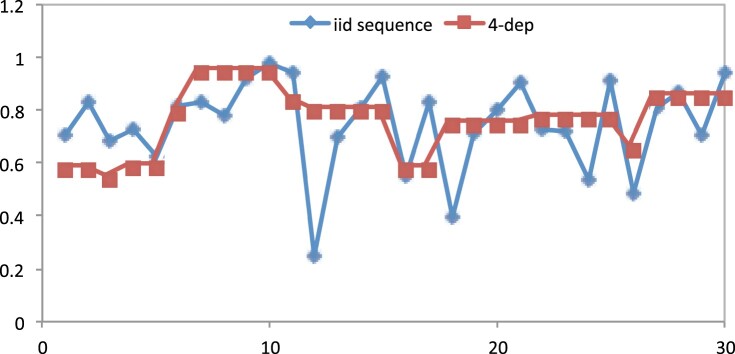
Figure 2 shows one realization of the process [M1] and of $Z_n$. Four-sized clusters of exceedances of high levels can be seen when $X_n$ is plotted, while for $Z_n$ only isolated values appear.

Figure 2.

One realization of an i.i.d. process and a 4-dependent moving maxima process.

The next example illustrates the behaviour of a stationary process for different values of EI.

Example 2.4 A Max-Autoregressive Process I, (Beirlant et al. [2]) —

Let $\{Y_n{\}}_{n\ge 1}$ be a sequence of i.i.d., unit-Fréchet. For $0<\theta \le 1$, let

$$[\mathrm{M}2]X_1=Y_1,X_n=max\{(1-\theta )X_{n-1},\theta Y_n\}n\ge 2.$$ (2)

For $u_n=nx$, x>0, $\mathbb{P}(M_{1,n}\le u_n)\to \exp (-\theta /x)$, as $n\to \mathrm{\infty }$,  so the EI of the sequence is θ, see Beirlant et al. [2].

Figure 3 shows partial realizations of the process [M2] with $\theta =0.1;0.5$ and 0.9, respectively. The maxima show increasing clustering as $\theta \to 0$. Notice also again a ‘shrinkage of maximum values’ as dependence increases.

Figure 3.

Samples of size n = 150 from M2 process, generated for $\theta =0.1$, $\theta =0.5$ and $\theta =0.9$.

Estimation of the EI is often based on the interpretation of θ due to Hsing et al. [14] as the reciprocal of the mean cluster size in the point process of exceedance times over a high threshold. Under a mixing condition which is slightly stronger than $D(u_n)$ those authors showed that the point process of exceedances converge weakly to a compound Poisson process, provided that $n\overline{F}(u_n(\tau ))\underset{n\to \mathrm{\infty }}{⟶}\tau$, i.e. $u_n(\tau )$ a normalized level. The distribution ${\pi }_n(j;u_n,r_n)$ of the cluster sizes is given by

$${\pi }_n(j;u_n,r_n)=\mathbb{P}\{\sum _{i=1}^{r_n}I(X_i>u_n)=j|\sum _{i=1}^{r_n}I(X_i>u_n)>0\},$$

for $j=1,\dots ,r_n$, $r_n\to \mathrm{\infty }$ and $r_n=o(n)$, and $I(.)$ denoting the indicator function. Under additional summability conditions on the ${\pi }_n$,

$$\sum _{j\ge 1}j{\pi }_n(j;u_n,r_n)\underset{n\to \mathrm{\infty }}{⟶}{\theta }^{-1},$$

i.e. the limiting mean number of exceedances of $u_n$ in an interval of length $r_n$ corresponds to the arithmetic inverse of the EI. So, we can write,

$${\theta }^{-1}=\sum _{j\ge 1}j\pi (j),$$

i.e. the mean cluster size in the limiting point process of exceedance times over high thresholds. This suggest that a suitable way to estimate the EI is to identify clusters of high levels exceedances, and to calculate the mean size of these clusters. By the way in which clusters are identified, the estimators fall apart in two types: blocks estimator and runs estimator (Smith and Weissman [26]; Weissman and Novak [28]; Hsing [13]). These estimators usually depend on two quantities to be chosen by the statistician: a threshold sequence and a cluster identification scheme parameter, such as the block size or the run length. In addition to the runs and blocks estimators of EI, two other estimators have recently been proposed: a two-threshold method (Laurini and Tawn [15]), and the intervals-estimator (Ferro and Segers [12]). The two-threshold method requires the choice of two declustering parameters. In contrast, inter-exceedance type estimators are attractive since they only depend on a threshold sequence.

Statistical properties, such as consistence and asymptotic distributional behaviour of those estimators are well documented in the aforementioned papers.

3. The blocks method to define clusters of exceedances

The blocks method consists of partitioning the n observations into consecutive $k_n=[n/r_n]$ contiguous blocks of a certain length, $r_n=o(n)$. In each block, the number of exceedances over a certain high threshold $u_n$ are counted, and the blocks estimator is then defined as the reciprocal of the average number of exceedances per block among blocks with at least one exceedance, defined by,

$${\hat{\theta }}_n^B(u_n):=\frac{\sum _{j=1}^{k_n}I(M_{(i-1)r_n,i{r}_n}>u_n)}{\sum _{i=1}^{n}I(X_i>u_n)}.$$ (3)

This blocks estimator of the EI has been intensively studied in the literature. Hsing [13] and Weissman and Novak [28] proved its consistency and asymptotic normality under suitable mixing conditions.

Variants of the blocks estimator were also examined by Smith and Weissman [26] and Robert et al. [23]. Blocks estimators can be constructed considering continuous blocks or sliding blocks. The asymptotic properties for both procedures were studied and compared in Robert et al. [23]. However, for both procedures the blocks estimator requires the choice of a threshold, $u_n$, and a block size, $r_n$. But, the behaviour of the estimates depend strongly of $r_n$ and $u_n$. Some recent works trying to deal with that situation can be mentioned, such as Berghaus and Bücher [3], Drees ([9,10]) and Northop [21].

Let us consider some other models that will be used in the simulation study to illustrate how the estimates depend on $r_n$ and $u_n$.

Example 3.1 A Max-Autoregressive Process II, (Alpuim [1]) —

Let $\{Y_n{\}}_{n\ge 1}$ be a sequence of independent, unit-Fréchet distributed random variables and $X_0$ a random variable with d.f. $H_0(x)=\exp (-x^{-1}({\beta }^{-1}-1))$. For $0<\beta <1$, let

$$[\mathrm{M}3]X_n=\beta max\{X_{n-1},Y_n\},n\ge 2.$$ (4)

The EI of this process is $\theta =1-\beta$, see Alpuim [1].

Example 3.2 A Second order autoregressive process, (Süveges [27]) —

Let $\{Y_n{\}}_{n\ge 1}$ be a sequence of independent, unit-Fréchet distributed random variables. Let $\{X_n{\}}_{n\ge 1}$ be the second order autoregressive process, defined as

$$[\mathrm{M}4]X_n=0.93X_{n-1}-0.86X_{n-2}+Y_n,n\ge 3.$$ (5)

The EI of this process is approximately 0.23, see Süveges [27].

Example 3.3 A Stochastic process, (Smith and Weissman [26]) —

Let $\{{\alpha }_n{\}}_{n\ge 1}$ be independent, distributed Bernoulli random variables with $\mathbb{P}\{{\alpha }_n=1\}=1-\mathbb{P}\{{\alpha }_n=0\}=\theta$ and $\{Y_n{\}}_{n\ge 1}$ be independent and identically distributed random variables, also independent of $\{{\alpha }_n\}$. The process $\{X_n{\}}_{n\ge 1}$ is defined as follows:

$$[\mathrm{M}5]X_1=Y_1,X_n={\alpha }_n{Y}_n+(1-{\alpha }_n)X_{n-1},n\ge 2.$$ (6)

The marginal d.f. of $\{X_n\}$ is F, the cluster sizes have geometric distribution with mean $1/\theta$, hence the EI of this process is θ, see Smith and Weissmank [26].

Example 3.4 A Max-Autoregressive Process III, (Smith [25]) —

Let $\{Y_n{\}}_{n\ge 1}$ be a sequence of independent, standard Gumbel distributed random variables. For fixed α define

$$[\mathrm{M}6]X_n=max\{X_{n-1}-\alpha ,Y_n+\log (1-\exp (-\alpha ))\}n\ge 1.$$ (7)

The EI of this process is $\theta =1-\exp (-\alpha )$, see Smith [25].

Example 3.5 A Moving Autoregressive process of order 2, (Reiss and Thomas [22]) —

Let $\{Y_n{\}}_{n\ge 1}$ be a sequence of independent, Pareto distributed random variables with tail index $\alpha >0$. Define

$$[\mathrm{M}7]X_n=Y_n+a_1{Y}_{n-1}+a_2{Y}_{n-2},n\ge 3.$$ (8)

The EI of this process is $\theta =1/(1+a_1^{\alpha }+a_1^{\alpha })$, see Reiss and Thomas [22].

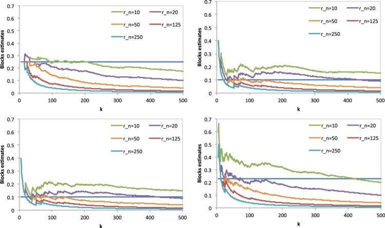
Figures 4 and 5 display blocks EI-estimates based on exceedances over a high threshold $u_n=X_{n-k:n}$, where $X_{1:n}\le X_{2:n}\le \dots \le X_{n:n}$ are the ascending order statistics (o.s.), associated to the sample $(X_1,X_2,\dots ,X_n)$. For each process [M1-M7] a sample of size n = 1000 was generated and the estimates were calculated for several block lengths, $r_n$.

Figure 4.

Estimates of ${\hat{\theta }}_n^B$ plotted against k ($u_n=X_{n-k:n}$), of a sequence of length n = 1000, with block lengths $r_n=10,20,50,125,250$, for the [M1] process (upper left), [M2] process (upper right), [M3] process (lower left) and [M4](lower right).

Figure 5.

Estimates of ${\hat{\theta }}_n^B$ plotted against k ($u_n=X_{n-k:n}$), of a sequence of length n = 1000, with block lengths $r_n=10,20,50,125,250$, for the [M5] process (left), [M6] process (center), [M7] process (right).

The estimates are almost monotones functions in $u_n$ and monotonically decreasing when the block lengths $r_n$ increases. It seems difficult to decide what $r_n$ should be chosen, there is some block size for which the path estimates do not cross the true value of the parameter. On the other hand the region of EI-estimates that shows some stability around the true value of the parameter depends on $r_n$ and even for a given $r_n$, it is not obvious how to choose the threshold appropriately.

4. A new approach for the blocks method estimator

We will consider here an estimator, introduced in Canto e Castro [5] who suggested a different approach to define the threshold inside each block. This approach works under a local dependence condition, $D^{(2)}(u_n)$, of Chernick et al. [6] based on Leadbetter and Nandagopalan [17] results. $D^{(2)}(u_n)$ condition, restricting rapid oscillations at high levels, requires the validity of the dependence condition $D(u_n)$ and is defined as:

Definition 4.1

Let $\{X_n{\}}_{n\ge 1}$ be a stationary sequence of random variables. $D^{(2)}(u_n)$ is said to be satisfied if

$$n\mathbb{P}\{X_j>u_n,X_{j+1}\le u_n,M_{j+2,r_n}>u_n\}\underset{n\to \mathrm{\infty }}{⟶}0,$$ (9)

with $u_n$ verifying the $D(u_n)$ condition and a sequence $r_n$ of block sizes such that $n/r_n\to \mathrm{\infty }$ and $r_n=o(n)$.

This condition locally restricts the occurrence of two or more upcrossings, but still allows clustering of exceedances.

The proposed estimator, Canto e Castro [5], was defined in the following way: let $k_n$ denote the number of blocks, and $r_n$ the respective block size. Let $v_{ni}$ be a sequence of levels such that

$$r_n\mathbb{P}\{X_1\le v_{ni}<X_2\}\underset{n\to \mathrm{\infty }}{⟶}1.$$ (10)

Denoting $N_i(r_n,v_{ni})$ as the number of up-crossing of $v_{ni}$ in $ith$ block, the estimator is defined by

$${\tilde{\theta }}_n^B(r_n):=\frac{k_n}{\sum _{i=1}^{k_n}{N}_i(r_n,v_{ni})}.$$ (11)

The properties of the estimator ${\tilde{\theta }}_n^B(r_n)$, in (11), were studied in Canto e Castro [5] and here will be presented the Theorems therein included. Let us first recall some notations:

• Leadbetter and Nandagopalan [17] showed that, under regular conditions, the point process of up-crossings

  $${\tilde{N}}_n(B)=\sum _{i=1}^n{ϵ}_{i/n}(B)I(X_{i-1}\le u_n<X_i),B\subset [0,1]$$

  converges to a Poisson point process with intensity that depends on the level $u_n$ and θ.
• Let $\mu (u)$ denotes the probability of a up-crossing can occur (not depending on the instant j due to the stationarity)

  $$\mu (u)=\mathbb{P}\{X_i\le u<X_{j+1}\}=\mathbb{P}\{X_j\le u|X_{j+1}>u\}\mathbb{P}\{X_{j+1}>u\}$$ (12)

The following Theorems that present conditions for consistence and the asymptotic normality of the estimator ${\tilde{\theta }}_n^B(r_n)$, in (11) are due to Canto e Castro [5] and there can be found the respective proves.

Theorem 4.2

Let $\{X_n{\}}_{n\ge 1}$ be a stationary sequence of random variables that satisfies $D(u_n)$ and $D^{(2)}(u_n)$ conditions for a sequence of levels $u_n$ such that $n\mu (u_n)\underset{n\to \mathrm{\infty }}{⟶}\nu$.

Then $\widetilde{N_n}\underset{n\to \mathrm{\infty }}{⟶}\tilde{N}$, where $\tilde{N}$ is a Poisson process in $[0,1]$ with intensity ν.

If, further, $\{X_n{\}}_{n\ge 1}$ has extremal index θ, then

$$n\mu (u_n)\underset{n\to \mathrm{\infty }}{⟶}\nu \text{if and only if}n\mathbb{P}\{X_1>u_n\}\underset{n\to \mathrm{\infty }}{⟶}\nu /\theta .$$

Theorem 4.3

Let $k_n$ be a sequence of positive numbers such that $k_n\to \mathrm{\infty }$ and $r_n=[n/k_n]$. Let us suppose that the stationary sequence of random variables, $\{X_n{\}}_{n\ge 1},$ has extremal index θ and satisfies $D(v_n)$ and $D^{(2)}(v_n)$ conditions, and that exists $l_n$ such that $k_n[{\alpha }_n(l_n-2,v_n)+\mathbb{P}\{M_{1,l_n}>v_n\}]\underset{n\to \mathrm{\infty }}{⟶}0$, for levels $v_n$ such that $r_n\mu (v_n)\underset{n\to \mathrm{\infty }}{⟶}1$, then

$${\displaystyle \frac{\sum _{i=1}^{k_n}{N}_i(r_n,v_n)}{k_n}}\underset{n\to \mathrm{\infty }}{⟶}\frac{1}{\theta }.$$

Theorem 4.4

If conditions established in Theorem 4.3 hold for levels $v_{n_i}$ such that $r_n\mu (v_{n_i})\underset{n\to \mathrm{\infty }}{⟶}1$, $i=1,\dots ,k_n$, then the estimator ${\tilde{\theta }}_n^B(r_n)$ is consistent.

Theorem 4.5

In conditions established in Theorem 4.3, if $E(N^2(r_n,v_n))\underset{n\to \mathrm{\infty }}{⟶}{c}^2(<\mathrm{\infty })$, and if, for each $ϵ>0,$ $k_{n}E(N^2(r_n,v_n)I(N^2(r_n,v_n)>ϵ))\underset{n\to \mathrm{\infty }}{⟶}0$ $($Lindeberg's condition$),$ for levels $v_n$ such that $r_n\mu (v_n)\underset{n\to \mathrm{\infty }}{⟶}1,$ then

$$k_n^{-1/2}(\sum _{i=1}^{k_n}{N}_i(r_n,v_n)-k_{n}E(N(r_n,v_n)))\stackrel{d}{⟶}N(0,\frac{1}{\theta }\sqrt{{\theta }^2{c}^2-1}).$$

Theorem 4.6

Suppose in addition to the conditions of Theorem 4.5 that

$$\sqrt{k_n}(N_i(r_n,v_n)-N_i(r_n,v_{ni}))\stackrel{p}{⟶}0$$

for levels $v_{ni}$ such that $r_n\mu (v_{ni})\underset{n\to \mathrm{\infty }}{⟶}1,$ $i=1,\dots ,k_n,$ then

$$\sqrt{k_n}({\tilde{\theta }}_n^B(r_n)-{\theta }_n)\stackrel{d}{⟶}N(0,\theta \sqrt{{\theta }^2{c}^2-1}),$$

where ${\theta }_n=(E(N(r_n,v_n)){)}^{-1}$.

Theorem 4.7

Suppose in addition to the conditions of Theorem 4.6 that

$${\theta }_n=\theta +o\left(\frac{1}{\sqrt{k_n}}\right).$$

Then

$$\sqrt{k_n}({\tilde{\theta }}_n^B(r_n)-\theta )\stackrel{d}{⟶}N(0,\theta \sqrt{{\theta }^2{c}^2-1}).$$

The estimator in (11) depends on the validity of $D^{(2)}(u_n)$ condition, that can be checked by calculating the proportion of the anti-$D^{(2)}(u_n)$ events $\{X_{j+1}\le u_n,M_{j+2,r_n}>u_n|X_j>u_n\}$ among the exceedances for a range of thresholds and block sizes, given $u_n$ and $r_n$, see Süveges [27], given by

$$p(u_n,r_n)=\frac{\sum _{j=1}^{n}I(X_j>u_n,X_{j+1}\le u_n,M_{j+2,r_n}>u_n)}{\sum _{j=1}^{n}I(X_j>u_n)},$$ (13)

for the observed sequence $\{X_1,\dots ,X_n\}$.

Examples are given in Figures 6–8 with [M1] process satisfying condition $D^{(2)}(u_n)$, with very low values of $p(u_n,r_n)$. However [M2], [M3], [M5], [M6] and [M7] processes depend on value of θ, showing higher values of $p(u_n,r_n)$ for high values of θ and small values of $p(u_n,r_n)$ for small values of θ.

Figure 6.

The observed proportions of $p(u_n,r_n)$ for the [M1–M3] process with $r_n=100$ (from left to right).

Figure 7.

The observed proportions of $p(u_n,r_n)$ for the [M4–M6] process with $r_n=100$ (from left to right).

Figure 8.

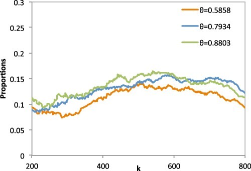
The observed proportions of $p(u_n,r_n)$ for the [M7] process with $r_n=100$.

Indeed processes [M2], [M3] and [M6] which are a special case of the general MARMA(p,q) processes introduced by Davis and Resnick [7] satisfies condition (9) for small values of θ, see Ferreira [11] and Martins and Sebastião [19]. Process [M4] does not verify that condition, see Süveges [27].

To apply this estimator to a given sample the $v_{ni}$ levels should be chosen verifying $r_{n}P\{X_1\le v_{ni}<X_2\}\sim 1.$ However the joint distribution of $(X_1,X_2)$ is unknown and so the $v_{ni}$ is. Under the validity of the $D^{(2)}(u_n)$ condition, it seems reasonable to substitute $v_{ni}$, in each block, by adequate levels such that the number of up-crossings is equal to 1, but low enough to identify exceedances. More precisely, we can define,

$$V_{ni}=inf\{u:N_i(r_n,u)=1\},i=1,\dots ,k_n.$$ (14)

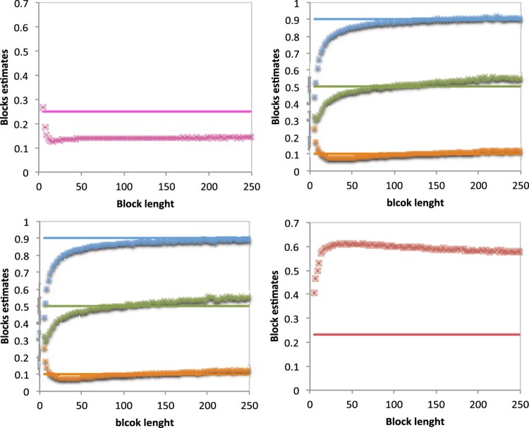
For each of processes (even for process [M4], for which we know that $D^{(2)}(u_n)$ condition is not verified) a n = 1000 sample-sized was generated and the estimator in (11) was applied. Figures 9 and 10 display the estimates obtained in each process for several values of block length.

Figure 9.

Estimates of ${\tilde{\theta }}_n^B$ of a sequence of length n = 1000, for different blocks lengths, from the [M1] process, (upper left); [M2] process (upper right); [M3] process (lower left) and [M4] process (lower right).

Figure 10.

Estimates of ${\tilde{\theta }}_n^B$ of a sequence of length n = 1000, for different blocks lengths, from the [M5] process, (left); [M6] process (middle); [M7] process (right).

For processes [M2], [M3] and [M6] the procedure presents very good results, a large stability region, very close to the true value of the parameter. It seems that we can consider the small value for $r_n$ for which a stability of the estimates path is obtained, and to estimate θ using that value of $r_n$.

For the [M4] process, for which the $D^{(2)}(u_n)$ condition is not verified, the stability region stays very far away from the true value of the parameter.

5. A choice of $r_n$: an heuristic sample path stability criterion

A path stability algorithm, see Caeiro and Gomes [4] and Neves et al. [20] has revealed quite nice results for extreme value parameters estimation and can now be adapted to the choice of $r_n$ and to obtain a θ estimate. Let us see the description of the algorithm, for ${\tilde{\mathrm{\Theta }}}^B(r_n)$ estimator:

1. Given an observed sample $(x_1,\dots ,x_n)$, compute the observed values of ${\tilde{\mathrm{\Theta }}}^B(r_n)$ for a range of values of $r_n$ (in our simulations we have considered $[n/100]⩽r_n⩽[n/4]$).

2. Obtain the rounded values, to 0 decimal places, of the estimates in the previous step. Define $a^{{\tilde{\theta }}^B(r_n)}(0)=\mathrm{round}({\tilde{\theta }}^B(r_n),0)$, $[n/100]⩽r_n⩽[n/4]$, the rounded values of ${\tilde{\mathrm{\Theta }}}^B(r_n)$ to 0 decimal places.

3. Consider the sets of r values associated to equal consecutive values of $a^{{\tilde{\theta }}^B(r_n)}(0)$, obtained in Step 2. Set $r_{min}^{{\tilde{\theta }}^B}$ and $r_{max}^{{\tilde{\theta }}^B}$ the minimum and maximum values, respectively, of the set with the largest range. The largest run size is then $l_{\theta }:=r_{max}^{{\tilde{\theta }}^B}-r_{min}^{{\tilde{\theta }}^B}$.

4. Consider all estimates, ${\tilde{\theta }}^B(r_n)$, for $r_{min}^{{\tilde{\theta }}^B}\le r_n\le r_{max}^{{\tilde{\theta }}^B}$, now with two extra decimal places, i.e. compute ${\tilde{\theta }}^B(r_n)=a_k^{{\tilde{\theta }}^B}(2)$. Obtain the mode of ${\tilde{\theta }}^B(r_n)$ and denote ${\mathcal{R}}_{{\tilde{\theta }}^B}$ the set of r-values associated with this mode.

5. Take $r_{n0}$ as the maximum value of ${\mathcal{R}}_{{\tilde{\theta }}^B}$, and consider the adaptive estimate ${\tilde{\theta }}^B(r_{n0})$.

6. The best estimate is the value of ${\tilde{\mathrm{\Theta }}}^B$ that corresponds to the maximum run size $l_{\theta }$ computed in Step 3.

Table 1 present the result of an application of the algorithm to samples generated from models [M1–M7], with the choice of $r_n$, $r_{n0}$, and the associated estimates.

Table 1. Values of $r_{n0}$ and the best estimates, ${\tilde{\theta }}^B(r_{n0})$, for samples simulated from models [M1–M7], and n = 500, 1000, 2000, 5000 samples-sized.

		n = 500		n = 1000		n = 2000		n = 5000
Models	θ	$r_{n0}$	${\tilde{\theta }}^B(r_{n0})$	$r_{n0}$	${\tilde{\theta }}^B(r_{n0})$	$r_{n0}$	${\tilde{\theta }}^B(r_{n0})$	$r_{n0}$	${\tilde{\theta }}^B(r_{n0})$
M1	0.25	95	0.1405	245	0.1423	490	0.1424	1200	0.1428
M2	0.1	90	0.1017	155	0.1086	195	0.1005	995	0.1204
	0.5	85	0.5219	190	0.5257	315	0.5395	445	0.5188
	0.9	105	0.9	200	0.9	395	0.9089	830	0.9117
M3	0.1	90	0.1071	195	0.1121	320	0.1131	995	0.1174
	0.5	65	0.5053	120	0.5144	270	0.5174	550	0.5266
	0.9	95	0.8668	240	0.8986	355	0.9027	1225	0.9116
M4	0.23	105	0.608	60	0.6076	425	0.5568	1245	0.5386
M5	0.1	70	0.0418	135	0.0491	495	0.0584	1225	0.0596
	0.5	75	0.3421	240	0.3748	230	0.3436	520	0.3476
	0.9	45	0.7855	245	0.8931	385	0.848	1055	0.8392
M6	0.1813	115	0.2131	195	0.2045	255	0.193	990	0.2125
	0.5034	60	0.5044	95	0.5106	220	0.5182	680	0.5345
	0.9093	80	0.8913	225	0.9133	420	0.9149	815	0.9186
M7	0.5858	90	0.6891	150	0.6896	390	0.7235	995	0.7208
	0.7934	35	0.837	120	0.9333	265	0.9667	1140	0.9297
	0.8803	85	0.8357	190	0.881	385	0.8973	1030	0.9289

6. An application

The data under study refers to the daily mean flow discharge rate values (${\mathrm{m}}^3/\mathrm{s}$) from 1 October, 1946 to 30 April, 2012 (‘SNIRH: Sistema Nacional de Informação dos Recursos Hídricos’). After some previous studies the stationarity of the data can be assumed from November until April (n = 11947).

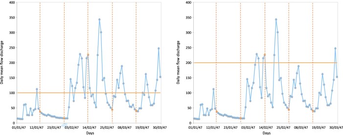
Figure 11 illustrates the effect of considering different thresholds, when the block length was fixed as $r_n=15$, for defining the clusters of exceedances, plotting a subset of the dataset available while Figure 12 displays the obtention of clusters, applying procedure (14) and considering three blocks, for the same subset used in Figure 11.

Figure 11.

Daily mean flow discharge rate values (${\mathrm{m}}^3/\mathrm{s}$) from 1 January 1947 to 30 March 1947 from hydrometric station at Fragas da Torre.

Figure 12.

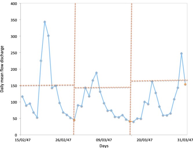
Daily mean flow discharge rate values (${\mathrm{m}}^3/\mathrm{s}$) from 1 January 1947 to 30 March 1947 from hydrometric station at Fragas da Torre.

We also checked the proportion of the anti-$D^{(2)}(u_n)$ events in our data and we verify that satisfies condition $D^{(2)}(u_n)$, see Figure 13.

Figure 13.

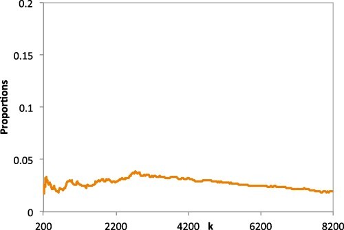
The observed proportions of $p(u_n,r_n)$ for the daily mean flow discharge rate values with $r_n=100$.

Figure 14 presents sample paths for the block-method EI- estimates. The difficulties of choosing the block size, $r_n$, as well as of choosing the adequate level k, are clear on the left plot of this figure.

Figure 14.

Estimates of ${\hat{\theta }}_n^B$ plotted against k ($u_n=X_{n-k:n}$) (left) and estimates of ${\tilde{\theta }}_n^B$ plotted against block length (right) with the choice of $r_n$ for the daily mean flow discharge rate values.

The right plot of Figure 14 presents the application of estimator (11). The application of the stability algorithm led to a block length $r_{n0}=975$ and an EI-estimate equal to 0.9231.

7. A few comments

The extremal index estimation is still an issue that needs some more research. Although some estimators have been recently proposed, the problem of choosing the threshold and/or the block or run length is not completely solved.

With the proposed estimator, the problem of the threshold choice is solved and here was proposed to consider a stability criterion for the choice of the block size and the corresponding estimate.

This is a preliminary approach for trying to consider a more reliable extremal index estimation procedure.

Funding Statement

This work has been supported by National Funds through FCT Fundação para a Ciência e a Tecnologia, Portugal, through the projects UID/MAT/00006/2019 (CEA/UL), UID/MAT/00297/2019 and UIDB/00297/2020.

Disclosure statement

No potential conflict of interest was reported by the author(s).

References

- 1.Alpuim M.T., An extremal Markovian sequence, J. Appl. Probab. 26 (1989), pp. 219–232. doi: 10.2307/3214030 [DOI] [Google Scholar]
- 2.Beirlant J., Goegebeur Y., Segers J., and Teugels J.L., Statistics of Extremes. Theory and Applications, 1st ed., John Wiley and Sons, England, 2004. [Google Scholar]
- 3.Berghaus B. and Bucher A., Weak convergence of a pseudo maximum likelihood estimator for the extremal index, Ann. Stat. 46 (2018), pp. 2307–2335. doi: 10.1214/17-AOS1621 [DOI] [Google Scholar]
- 4.Caeiro F. and Gomes M.I., Threshold selection in extreme value analysis, in Extreme Value Modeling and Risk Analysis: Methods and Applications, Dipak Dey and Jun Yan, eds., Chapman-Hall/CRC, Boca Raton, 2015, pp. 69–87.
- 5.Canto e Castro L., Estudo de um método de estimação do indice extremal, I Congresso Ibero-Americano de Estadística e Investigación Operativa, Salamandra,1992.
- 6.Chernick M.R., Hsing J.T., and McCormick W.P., Calculating the extremal index for a class of stationary sequences, Adv. Appl. Probab. 23 (1991), pp. 835–850. doi: 10.2307/1427679 [DOI] [Google Scholar]
- 7.Davis R.A. and Resnick S.I., Basic properties and prediction of Max-ARMA processes, Adv. Appl. Probab. 21 (1989), pp. 781–803. doi: 10.2307/1427767 [DOI] [Google Scholar]
- 8.Díaz-Delgado R., Lloret F., and Pons X., Spatial patterns of fire occurrence in Catalonia, NE, Spain, Landscape Ecol. 19 (2004), pp. 731–745. doi: 10.1007/s10980-005-0183-1 [DOI] [Google Scholar]
- 9.Drees H., Bias correction for estimators of the extremal index, preprint (2011), submitted for publication. Available at https://arxiv.org/abs/1107.0935.
- 10.Drees H., Extreme quantile estimation for dependent data with applications to finance, Bernoulli 9 (2003), pp. 617–657. doi: 10.3150/bj/1066223272 [DOI] [Google Scholar]
- 11.Ferreira M., Heuristic tools for the estimation of the extremal index: A comparison of methods, REVSTAT – Stat. J. 16 (2018), pp. 115–136. [Google Scholar]
- 12.Ferro C.A.T. and Segers J., Inference for clusters of extreme values, J. R. Stat. Soc. Ser. B 65 (2003), pp. 545–556. doi: 10.1111/1467-9868.00401 [DOI] [Google Scholar]
- 13.Hsing J.T., Extremal index estimation for a weakly dependent stationary sequence, Ann. Stat. 21 (1993), pp. 2043–2071. doi: 10.1214/aos/1176349409 [DOI] [Google Scholar]
- 14.Hsing J.T., Hüsler J., and Leadbetter M.R., On the exceedance point process for a stationary sequence, Probab. Theory Relat. Fields 78 (1988), pp. 97–112. doi: 10.1007/BF00718038 [DOI] [Google Scholar]
- 15.Laurini F. and Tawn J.A., New estimators for the extremal index and other cluster characteristics, Extremes 6 (2003), pp. 189–211. doi: 10.1023/B:EXTR.0000031179.49454.90 [DOI] [Google Scholar]
- 16.Lavanda B. and Cipollone E., Extreme value statistics and thermodynamics of earthquakes: Aftershock sequences, Ann. Geofis. 43 (2000), pp. 967–982. [Google Scholar]
- 17.Leadbetter M.R. and Nandagopalan L., On exceedance point process for stationary sequences under mild oscillation restrictions, in Extreme Value Theory: Proceedings, Lecture Notes in Statistics 52, Oberwolfach, J. Hüsler and R. D. Reiss, eds., Springer-Verlag, Berlim, 1989, pp. 69–80.
- 18.Leadbetter M.R., Lindgren G., and Rootzén H., Extremes and Related Properties of Random Sequences and Series, Springer-Verlag, New York, 1983. [Google Scholar]
- 19.Martins A.P. and Sebastião J.R., Methods for estimating the upcrossings index: Improvements and comparison, Stat. Papers 60 (2017), pp. 1317–1347. doi: 10.1007/s00362-017-0876-x [DOI] [Google Scholar]
- 20.Neves M.M., Gomes M.I., Figueiredo F., and Gomes D.P., Modelling extreme events: Sample fraction adaptive choice in parameter estimation, J. Stat. Theory Practice 9 (2015), pp. 184–199. doi: 10.1080/15598608.2014.890984 [DOI] [Google Scholar]
- 21.Northrop P.J., An efficient semiparametric maxima estimator of the extremal index, Extremes 18 (2005), pp. 585–603. doi: 10.1007/s10687-015-0221-5 [DOI] [Google Scholar]
- 22.Reiss R.-D. and Thomas M., Statistical Analysis of Extreme Values: With Applications to Insurance, Finance, Hydrology and Other Fields, 3rd ed., Birkhäuser Verlag, Basel, 2007. [Google Scholar]
- 23.Robert C.Y., Segers J., and Ferro C.A.T., A sliding blocks estimator for the extremal index, E. J. Stat. 3 (2009), pp. 993–1020. doi: 10.1214/08-EJS345 [DOI] [Google Scholar]
- 24.Schoenberg F.P., Peng R., Huang Z., and Rundel P., Detection of nonlinearities in the dependence of burn area on fuel age and climatic variables, Int. J. Wildland Fire 12 (2003), pp. 1–10. doi: 10.1071/WF02053 [DOI] [Google Scholar]
- 25.Smith R.L., The extremal index for a markov chain, J. Appl. Probab. 29 (1992), pp. 37–45. doi: 10.2307/3214789 [DOI] [Google Scholar]
- 26.Smith R. and Weissman I., Estimating the extremal index, J. R. Stat. Soc. B 56 (1993), pp. 515–528. [Google Scholar]
- 27.Süveges M., Likelihood estimation of the extremal index, Extremes 10 (2007), pp. 41–55. doi: 10.1007/s10687-007-0034-2 [DOI] [Google Scholar]
- 28.Weissman I. and Novak S.Y., On blocks and runs estimators of the extremal index, J. Stat. Plann. Inf. 66 (1998), pp. 281–288. doi: 10.1016/S0378-3758(97)00095-5 [DOI] [Google Scholar]