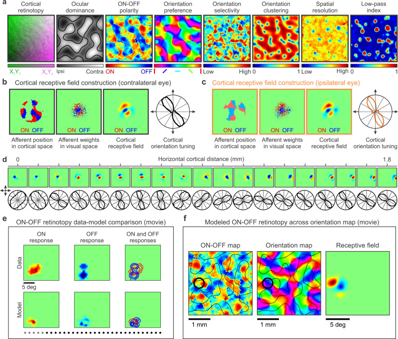
Fig. 6. Model outputs. Visual maps for multiple stimulus dimensions, cortical receptive fields and neuronal response properties.

a The model generates maps for multiple stimulus dimensions illustrated, from left to right, for retinotopy, ocular dominance, ONOFF polarity, orientation preference, orientation selectivity, orientation clustering, spatial resolution (highest spatial frequency generating half-maximum response), and low-pass index (response at lowest spatial frequency divided by maximum response). b The model output also provides the position in cortical space of the main afferent axons converging at the same cortical pixel (left square panel), the afferent receptive field positions and synaptic weights in visual space (middle square panel, dot position and size), and the cortical receptive field and orientation tuning resulting from afferent convergence (for the contralateral eye). c Same as (b) for the ipsilateral eye (notice the precise binocular match of orientation preference). d It also generates cortical receptive fields (top) and orientation tuning (bottom) for each pixel of the visual map. As in experimental measures²⁸, the receptive fields change with cortical distance in position (retinotopy), ONOFF dominance, orientation preference, and subregion structure (top). The orientation preference and orientation selectivity also changes systematically with cortical distance (bottom). e Model-data comparison of ON-OFF retinotopy changes with cortical distance (see movie Fig. 6e). The gray dots at the bottom illustrate the cortical pixels included in the receptive field average (average along a cortical distance of 400 microns, distance between pixels 100 microns). Notice that ONOFF retinotopy systematically changes along a diagonal line in visual space. However, the diagonal line is not straight; ON and OFF retinotopy move around and intersect with each other, as expected from ONOFF afferent sorting. f Model simulations illustrating the relation between ONOFF dominance (left), orientation preference (middle), and receptive field structure (right, see movie Fig. 6f).