Figure 5.

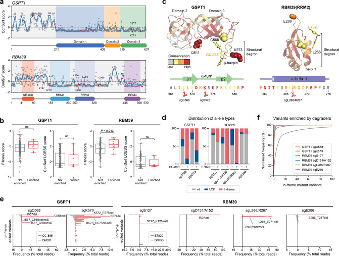
Resistance mutation sites across TPD targets exhibit low levels of sequence conservation. (a) ConSurf conservation scores (y axis) of amino acid residues in GSPT1 (top panel) and RBM39 (bottom panel) shown as dots with the LOESS regression line in blue. Amino acids corresponding to enriched sgRNA cut site positions from the CRISPR-suppressor scanning are highlighted in red and key residues are labeled. (b) Box plots with jitter showing fitness scores and ConSurf LOESS scores for nonenriched (gray, n = 230 for GSPT1 and 119 for RBM39) or enriched (red, n = 9 for GSPT1 and 10 for RBM39) sgRNAs. Fitness scores were calculated as the log₂(fold-change sgRNA enrichment at week 4 under vehicle treatment versus the plasmid library) normalized to the mean of the negative control sgRNAs. sgRNAs were assigned ConSurf LOESS scores based on the amino acid corresponding to their predicted cut site positions; sgRNAs cutting between amino acids were assigned the mean of the flanking amino acids’ scores. Dots represent the fitness scores or corresponding amino acid ConSurf LOESS scores for individual sgRNAs. Two-sided P values were calculated with the Mann–Whitney test (ns: not significant). The box shows the median, 25th, and 75th percentiles with whiskers denoting 1.5 × the interquartile range. (c) Structural view of GSPT1(I440-P634) (left) and RBM39(RRM2) (right), with residues colored according to ConSurf conservation scores. The top three most conserved bins of ConSurf scores are colored in red, orange, and yellow, respectively, and the bottom six bins are colored in gray. sgRNAs enriched in the CRISPR-suppressor scan are depicted as spheres. Sequences corresponding to the approximate region around the structural degrons are shown below and colored according to ConSurf scores. (d) Stacked bar plot showing the frequency distribution of variant types (y axis, % of total reads) after transduction of the indicated sgRNAs targeting GSPT1 and RBM39 and treatment with vehicle or drug molecules (see Methods) for four weeks. (e) Bar plots showing variant frequencies (x axis, % of total reads) for the top 50 variants (y axis) generated by the indicated sgRNAs after treatment with vehicle (gray bars, left) or drug molecules (red bars, right) for four weeks. Variants are rank-ordered on the y axis by decreasing frequency in vehicle treatment for each sgRNA. (f) Cumulative plot showing the normalized variant frequency (y axis) for the 100 most abundant in-frame edited variants (x axis) for each indicated sgRNA after drug treatment for four weeks. Variants are rank-ordered on the x axis by decreasing normalized frequency for each respective sgRNA condition. Variant frequency was normalized to the total frequency of all in-frame edited variants.