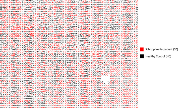
FIGURE 6.

A subset of dominant motifs from SZ and HC dynamics. The motifs are detrended and visualized using tSNE followed by the Jonker‐Volgenant algorithm for the linear assignment problems. A similar type of shape is embedded into the same neighborhood. We can see a few potential subgroups of motifs. The blank space in the figure was generated because we used a larger 2D grid than the number of motifs to display. So, the algorithm optimizes the location for each motif from the 2D coordinate system to assign the matching patterns in the nearby vicinity. The X axis is time, and the Y axis represents the dynamic functional connectivity strength