
Fig. 5.
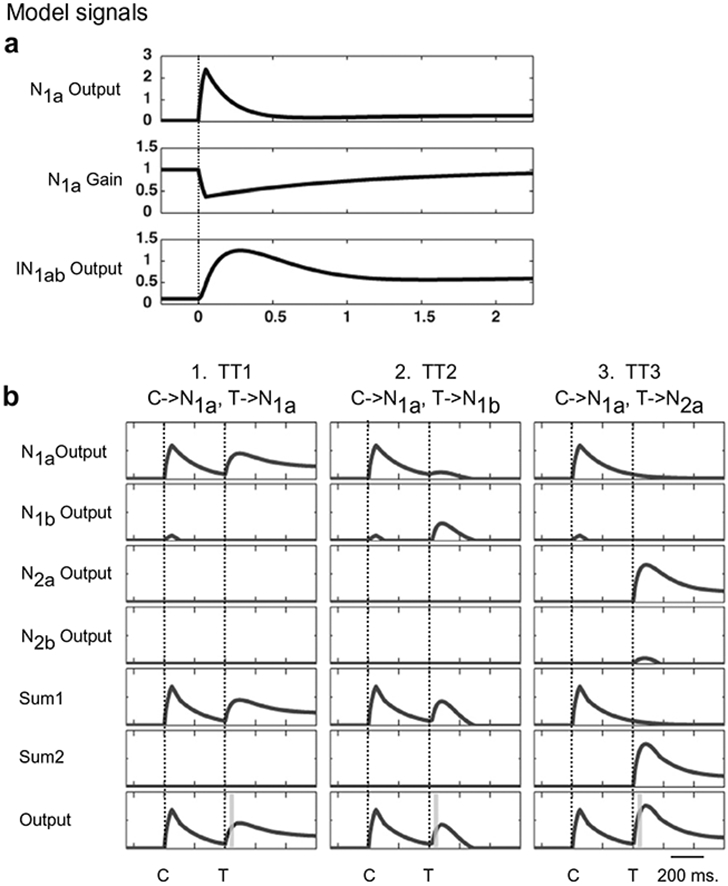
Simulated neuronal activity traces in response to a single pulse input simulating the presentation of shape “a” in location 1. (a) A 50 ms pulse is applied to N1a at time 0 (dotted vertical lines). The inputs to the other three neurons were set to zero. The top panel shows the firing rate output of N1a. Other shape selective neurons in the model have similar dynamic properties. It shows a rapid increase in firing rate followed by a slow decay to an elevated baseline. The middle panel shows the gain change that occurs within N1a for the excitatory input of N1a. The lower panel shows the firing rate changes in the inter-neuron IN1ab. (b) Responses of model neurons for a cue and a target presentation. Each column of traces represents one of three types of cueing protocol: column 1, TT1 – cue (C) and target (T) have same shapes and are presented at the same location (left column), column 2, TT2 – cue and target have different shapes but are presented at the same location (middle column), and column 3, TT3 – cue and target have same shapes but are presented at different locations (right column). The cue duration is 50 ms and CTOA is 400 ms. The target stays on until the end of simulation. The left (right) vertical dotted line in each column represents the onset of cue (target). The first four rows show the firing rates of N1a, N1b, N2a and N2b respectively. The following two rows show the summed activity for each encoded location (Sum1, Sum2). The output of the model is shown in the bottom row. The vertical gray bar in each column of the bottom row indicates the temporal window over which the model’s output is integrated for computations of the cueing effects presented in the following two figures.