Maximal rough neighborhoods with a medical application

Abstract

In this paper, we focus on the main concepts of rough set theory induced from the idea of neighborhoods. First, we put forward new types of maximal neighborhoods (briefly, ${\mathcal{M}}_{\sigma }$-neighborhoods) and explore master properties. We also reveal their relationships with foregoing neighborhoods and specify the sufficient conditions to obtain some equivalences. Then, we apply ${\mathcal{M}}_{\sigma }$-neighborhoods to define ${\mathcal{M}}_{\sigma }$-lower and ${\mathcal{M}}_{\sigma }$-upper approximations and elucidate which one of Pawlak’s properties are preserved (evaporated) by these approximations. Moreover, we research ${\mathcal{A}}_{M\sigma }$-accuracy measures and prove that they keep the monotonic property under any arbitrary relation. We provide some comparisons that illustrate the best approximations and accuracy measures are obtained when $\sigma =⟨i⟩$. To show the importance of ${\mathcal{M}}_{\sigma }$-neighborhoods, we present a medical application of them in classifying individuals of a specific facility in terms of their infection with COVID-19. Finally, we scrutinize the strengths and limitations of the followed technique in this manuscript compared with the previous ones.

Introduction

Pawlak (1982, 1991) familiarized the idea of rough sets theory as a mathematical tool to address incomplete information systems and uncertainty. The essential notions in this theory such as upper and lower approximations and accuracy measures are firstly characterized using an equivalence relation. In past few years, many novel models have been espoused, by changing or relaxing some underlying conditions.

After the superb start of studying rough sets using right and left neighborhoods (Yao 1996, 1998), some rough set models have been established such as minimal left neighborhoods (Allam et al. 2006) and minimal right neighborhoods (Allam et al. 2005). Then, intersection and union neighborhoods, intersection minimal and union minimal neighborhoods were introduced in (Abd El-Monsef et al. 2014). Generating right neighborhoods from finite class of arbitrary relations was investigated in (Abu-Donia 2008). Mareay (2016) studied four types of neighborhoods using the equality relation between ${\mathcal{N}}_{\sigma }$-neighborhoods. Sun et al. (2019) defined the dual idea of neighborhood systems under the name of remote neighborhood systems. Recently, Al-shami et al. (2021b) have applied the intersection operation between ${\mathcal{N}}_{\sigma }$-neighborhoods to define ${\mathcal{E}}_{\sigma }$-neighborhoods. Also, novel types of neighborhoods called ${\mathcal{C}}_{\sigma }$-neighborhoods (Al-shami 2021a) and ${\mathcal{S}}_{\sigma }$-neighborhoods (Al-shami and Ciucci 2022) have been initiated using the inclusion relation between ${\mathcal{N}}_{\sigma }$-neighborhoods.

Following this line of study, we display the concept of ${\mathcal{M}}_{\sigma }$-neighborhood systems. The motivations are twofold. From a theoretical standpoint, the lower and upper approximations satisfy most of the properties of the standard Pawlak model, and the accuracy measures preserve the monotonic property under any arbitrary relation as illustrated in Proposition 25 and Corollary 26. Whereas, this property is losing or keeping under strict conditions in some foregoing methods such as those introduced by Mareay (2016) and Al-shami (2021a). From an application prospective, ${\mathcal{M}}_{\sigma }$-neighborhood systems can be used in concrete situations as we explain in Sect. 5. Also, ${\mathcal{M}}_i$- and ${\mathcal{M}}_{⟨i⟩}$-neighborhoods improve the approximations and accuracy measures more than ${\mathcal{M}}_r$-neighborhoods given by Dai et al. (2018).

The arrangement of the rest of this manuscript is as follows. Sect. 2 reviews the literature needed to understand the article’s results. In Sect. 3, we embraced a new class of neighborhoods system called ${\mathcal{M}}_{\sigma }$-neighborhoods, where $\sigma \in \{l,⟨r⟩,⟨l⟩,i,u,⟨i⟩,⟨u⟩\}$. In Sect. 4, we mainly aim to introduce different types of approximations and accuracy measures. We compare between them and elucidate that the best case given by $⟨i⟩$. In Sect. 5, we propose an algorithm to classify the individuals who work in a specific facility with respect to corona-virus COVID-19 infection. Finally, discussions and conclusions are provided in Sects. 6 and 7, respectively.

Preliminaries

In this section, we provide some definitions and results of different types of neighborhoods to make this manuscript self-contained and also to rationalize the need to introduce the concept of ${\mathcal{M}}_{\sigma }$-neighborhoods.

Definition 1

(see, Abd El-Monsef et al. 2014) A binary relation $\theta$ on $\mathcal{B}$ is a subset of $\mathcal{B}\times \mathcal{B}$. We write $\alpha \theta \beta$ if $(\alpha ,\beta )\in \theta$.

$\theta$ is called reflexive (resp., symmetric, transitive) if $\alpha \theta \alpha$ for each $\alpha \in \mathcal{B}$ (resp., $\alpha \theta \beta ⟺\beta \theta \alpha$, $\alpha \theta \delta$ whenever $\alpha \theta \beta$ and $\beta \theta \delta$). If $\theta$ is reflexive, symmetric and transitive, then it called an equivalence relation. Also, we call $\theta$ a comparable relation if $\alpha \theta \beta$ or $\beta \theta \alpha$ for each $\alpha ,\beta \in \mathcal{B}$.

Definition 2

(Pawlak 1982, 1991) Let $\theta$ be an equivalence relation on $\mathcal{B}$. We associate every $W\subseteq \mathcal{B}$ with two subsets:

$\underset{\_}{\theta }(W)=\bigcup \{E\in \mathcal{B}/\theta :E\subseteq W\}$ (It is called the lower approximation of W).

$\overline{\theta }(W)=\bigcup \{E\in \mathcal{B}/\theta :E\bigcap W\ne \mathrm{\varnothing }\}$ (It is called the upper approximation of W)

The following result lists the core properties of Pawlak’s rough set model. In the previous generalized rough set models, the validity of these properties was examined. Of course, some of them are evaporated in these models; however, keeping as many as possible of these properties is considered as an advantage of the model.

Proposition 1

(Pawlak 1982, 1991) Let V, W be two subsets of $\mathcal{B}$. The following properties are satisfied if $\theta$ is an equivalence relation on $\mathcal{B}$.

1. $\underset{\_}{\theta }(V)\subseteq V$

2. $V\subseteq \overline{\theta }(V)$

3. $\underset{\_}{\theta }(\mathrm{\varnothing })=\mathrm{\varnothing }$

4. $\overline{\theta }(\mathrm{\varnothing })=\mathrm{\varnothing }$

5. $\underset{\_}{\theta }(\mathcal{B})=\mathcal{B}$

6. $\overline{\theta }(\mathcal{B})=\mathcal{B}$

7. $IfV\subseteq W$, then $\underset{\_}{\theta }(V)\subseteq \underset{\_}{\theta }(W)$

8. $IfV\subseteq W$, then $\overline{\theta }(V)\subseteq \overline{\theta }(W)$

9. $\underset{\_}{\theta }(V\cap W)=\underset{\_}{\theta }(V)\cap \underset{\_}{\theta }(W)$

10. $\overline{\theta }(V\cap W)\subseteq \overline{\theta }(V)\cap \overline{\theta }(W)$

11. $\underset{\_}{\theta }(V)\cup \underset{\_}{\theta }(W)\subseteq \underset{\_}{\theta }(V\cup W)$

12. $\overline{\theta }(V\cup W)=\overline{\theta }(V)\cup \overline{\theta }(W)$

13. $\underset{\_}{\theta }(V^c)={(\overline{\theta }(V))}^c$

14. $\overline{\theta }(V^c)={(\underset{\_}{\theta }(V))}^c$

15. $\underset{\_}{\theta }(\underset{\_}{\theta }(V))=\underset{\_}{\theta }(V)$

16. $\overline{\theta }(\overline{\theta }(V))=\overline{\theta }(V)$

17. $\underset{\_}{\theta }({(\underset{\_}{\theta }(V))}^c)={(\overline{\theta }(V))}^c$

18. $\overline{\theta }({(\overline{\theta }(V))}^c)={(\underset{\_}{\theta }(V))}^c$

19. $\forall X\in \mathcal{B}/\theta \Rightarrow \underset{\_}{\theta }(X)=X$

20. $\forall X\in \mathcal{B}/\theta \Rightarrow \overline{\theta }(X)=X$

We can also numerically describe rough sets by using the following two measures.

Definition 3

(Pawlak 1982, 1991) Let $\theta$ be an equivalence relation on $\mathcal{B}$. The $\mathcal{A}$-accuracy and $\mathcal{R}$-roughness measures of a nonempty subset W of $\mathcal{B}$ with respect to an equivalence relation $\theta$ are respectively defined by

$$\begin{array}{cc}\hfill \mathcal{A}(W)=& \frac{\mid \underset{\_}{\theta }(W)\mid }{\mid \overline{\theta }(W)\mid }.\hfill \\ \hfill \mathcal{R}(W)=& 1-\mathcal{A}(W).\hfill \end{array}$$

The equivalence relations are a strict condition and cannot be satisfied in many circumstances. So that, the classical model has been extended using weaker relations than the equivalence.

Definition 4

(Abd El-Monsef et al. 2014; Abo-Tabl 2011; Allam et al. 2005, 2006; Yao 1996, 1998) The ${\mathcal{N}}_{\sigma }$-neighborhoods of an $\alpha \in \mathcal{B}$ (denoted by ${\mathcal{N}}_{\sigma }(\alpha )$) are defined under an arbitrary relation $\theta$ on $\mathcal{B}$, where $\sigma \in \{r,l,⟨r⟩,⟨l⟩$, $i,u,⟨i⟩,⟨u⟩\}$, as follows.

• (i)${\mathcal{N}}_r(\alpha )=\{\beta \in \mathcal{B}:\alpha \theta \beta \}$.
• (ii)${\mathcal{N}}_l(\alpha )=\{\beta \in \mathcal{B}:\beta \theta \alpha \}$.
• (iii)
  $$\begin{array}{c}\hfill {\mathcal{N}}_{⟨r⟩}(\alpha )=\left\{\begin{array}{ccc}\bigcap _{\alpha \in {\mathcal{N}}_r(\beta )}{\mathcal{N}}_r(\beta )\hfill & :\hfill & \exists {\mathcal{N}}_r(\beta )\text{containing}\alpha \hfill \\ \mathrm{\varnothing }\hfill & :\hfill & Otherwise\hfill \end{array}\right)\end{array}$$
• (iv)
  $$\begin{array}{c}\hfill {\mathcal{N}}_{⟨l⟩}(\alpha )=\left\{\begin{array}{ccc}\bigcap _{\alpha \in {\mathcal{N}}_l(\beta )}{\mathcal{N}}_l(\beta )\hfill & :\hfill & \exists {\mathcal{N}}_l(\beta )\text{containing}\alpha \hfill \\ \mathrm{\varnothing }\hfill & :\hfill & Otherwise\hfill \end{array}\right)\end{array}$$
• (v)${\mathcal{N}}_i(\alpha )={\mathcal{N}}_r(\alpha )\bigcap {\mathcal{N}}_l(\alpha )$.
• (vi)${\mathcal{N}}_u(\alpha )={\mathcal{N}}_r(\alpha )\bigcup {\mathcal{N}}_l(\alpha )$.
• (vii)${\mathcal{N}}_{⟨i⟩}(\alpha )={\mathcal{N}}_{⟨r⟩}(\alpha )\bigcap {\mathcal{N}}_{⟨l⟩}(\alpha )$.
• (viii)${\mathcal{N}}_{⟨u⟩}(\alpha )={\mathcal{N}}_{⟨r⟩}(\alpha )\bigcup {\mathcal{N}}_{⟨l⟩}(\alpha )$.

Henceforth, we consider $\sigma \in \{r,l,⟨r⟩,⟨l⟩,i,u$, $⟨i⟩,⟨u⟩\}$, unless stated otherwise.

Definition 5

(Abd El-Monsef et al. 2014) Let $\theta$ be an arbitrary relation on $\mathcal{B}$ and ${\zeta }_{\sigma }$ be a map from $\mathcal{B}$ to $2^{\mathcal{B}}$ which associated each $\alpha \in \mathcal{B}$ with its $\sigma$-neighborhood in $2^{\mathcal{B}}$. We call the triple $(\mathcal{B},\theta ,{\zeta }_{\sigma })$ a $\sigma$-neighborhood space (briefly, $\sigma$-NS)

Definition 6

(Al-shami et al. 2021b) The $\mathcal{E}$-neighborhoods of an $\alpha \in \mathcal{B}$ (briefly, ${\mathcal{E}}_{\sigma }(\alpha )$) are defined for each $\sigma$ under an arbitrary relation $\theta$ on $\mathcal{B}$ as follows.

• (i)${\mathcal{E}}_r(\alpha )=\{\beta \in \mathcal{B}:{\mathcal{N}}_r(\beta )\bigcap {\mathcal{N}}_r(\alpha )\ne \mathrm{\varnothing }\}$.
• (ii)${\mathcal{E}}_l(\alpha )=\{\beta \in \mathcal{B}:{\mathcal{N}}_l(\beta )\bigcap {\mathcal{N}}_l(\alpha )\ne \mathrm{\varnothing }\}$.
• (iii)${\mathcal{E}}_i(\alpha )={\mathcal{E}}_r(\alpha )\bigcap {\mathcal{E}}_l(\alpha )$.
• (iv)${\mathcal{E}}_u(\alpha )={\mathcal{E}}_r(\alpha )\bigcup {\mathcal{E}}_l(\alpha )$.
• (v)${\mathcal{E}}_{⟨r⟩}(\alpha )=\{\beta \in \mathcal{B}:{\mathcal{N}}_{⟨r⟩}(\beta )\bigcap {\mathcal{N}}_{⟨r⟩}(\alpha )\ne \mathrm{\varnothing }\}$.
• (vi)${\mathcal{E}}_{⟨l⟩}(\alpha )=\{\beta \in \mathcal{B}:{\mathcal{N}}_{⟨l⟩}(\beta )\bigcap {\mathcal{N}}_{⟨l⟩}(\alpha )\ne \mathrm{\varnothing }\}$.
• (vii)${\mathcal{E}}_{⟨i⟩}(\alpha )={\mathcal{E}}_{⟨r⟩}(\alpha )\bigcap {\mathcal{E}}_{⟨l⟩}(\alpha )$.
• (viii)${\mathcal{E}}_{⟨u⟩}(\alpha )={\mathcal{E}}_{⟨r⟩}(\alpha )\bigcup {\mathcal{E}}_{⟨l⟩}(\alpha )$.

Definition 7

(Al-shami 2021a) The $\mathcal{C}$-neighborhoods of an $\alpha \in \mathcal{B}$ (briefly, ${\mathcal{C}}_{\sigma }(\alpha )$) are defined for each $\sigma$ under an arbitrary relation $\theta$ on $\mathcal{B}$ as follows.

• (i)${\mathcal{C}}_r(\alpha )=\{\beta \in \mathcal{B}:{\mathcal{N}}_r(\beta )\subseteq {\mathcal{N}}_r(\alpha )\}$.
• (ii)${\mathcal{C}}_l(\alpha )=\{\beta \in \mathcal{B}:{\mathcal{N}}_l(\beta )\subseteq {\mathcal{N}}_l(\alpha )\}$.
• (iii)${\mathcal{C}}_i(\alpha )={\mathcal{C}}_r(\alpha )\bigcap {\mathcal{C}}_l(\alpha )$.
• (iv)${\mathcal{C}}_u(\alpha )={\mathcal{C}}_r(\alpha )\bigcup {\mathcal{C}}_l(\alpha )$.
• (v)${\mathcal{C}}_{⟨r⟩}(\alpha )=\{\beta \in \mathcal{B}:{\mathcal{N}}_{⟨r⟩}(\beta )\subseteq {\mathcal{N}}_{⟨r⟩}(\alpha )\}$.
• (vi)${\mathcal{C}}_{⟨l⟩}(\alpha )=\{\beta \in \mathcal{B}:{\mathcal{N}}_{⟨l⟩}(\beta )\subseteq {\mathcal{N}}_{⟨l⟩}(\alpha )\}$.
• (vii)${\mathcal{C}}_{⟨i⟩}(\alpha )={\mathcal{C}}_{⟨r⟩}(\alpha )\bigcap {\mathcal{C}}_{⟨l⟩}(\alpha )$.
• (viii)${\mathcal{C}}_{⟨u⟩}(\alpha )={\mathcal{C}}_{⟨r⟩}(\alpha )\bigcup {\mathcal{C}}_{⟨l⟩}(\alpha )$.

The foregoing types of neighborhoods were applied to define new types of lower and upper approximations and accuracy (roughness) measures. Comparisons between them in terms of improving the approximations and increasing the accuracy measures were done in various papers.

Definition 8

(Abd El-Monsef et al. 2014; Abo-Tabl 2011; Allam et al. 2005, 2006; Al-shami 2021a; Al-shami et al. 2021b; Yao 1996, 1998) Let $\theta$ be an arbitrary relation on $\mathcal{B}$ and $\mathcal{K}\in \{\mathcal{N},\mathcal{E},\mathcal{C}\}$. We define lower and upper approximations of each $W\subseteq \mathcal{B}$ with respect to the types of neighborhoods as follows.

$$\begin{array}{cc}\hfill {\mathcal{H}}_{\mathcal{K}\sigma }(W)=& \{\alpha \in \mathcal{B}:{\mathcal{K}}_{\sigma }(\alpha )\subseteq W\},\text{and}\hfill \\ \hfill {\mathcal{H}}^{\mathcal{K}\sigma }(W)=& \{\alpha \in \mathcal{B}:{\mathcal{K}}_{\sigma }(\alpha )\bigcap W\ne \mathrm{\varnothing }\}.\hfill \end{array}$$

Definition 9

(Abd El-Monsef et al. 2014; Allam et al. 2005, 2006; Al-shami 2021a; Al-shami et al. 2021b; Yao 1996, 1998) Let $\theta$ be an arbitrary relation on $\mathcal{B}$. The ${\mathcal{A}}_{\mathcal{K}\sigma }$ and ${\mathcal{A}}_{\mathcal{C}\sigma }$-accuracy and ${\mathcal{R}}_{\mathcal{K}\sigma }$-roughness measures of a nonempty subset W of $\mathcal{B}$ with respect to $\theta$ are respectively defined by

$$\begin{array}{cc}\hfill {\mathcal{A}}_{\mathcal{K}\sigma }(W)=& \frac{\mid {\mathcal{H}}_{\mathcal{K}\sigma }(W)\bigcap W\mid }{\mid {\mathcal{H}}^{\mathcal{K}\sigma }(W)\bigcup W\mid },\mathcal{K}\in \{\mathcal{N},\mathcal{E}\}\text{and}\hfill \\ \hfill {\mathcal{A}}_{\mathcal{C}\sigma }(W)=& \frac{\mid {\mathcal{H}}_{\mathcal{C}\sigma }(W)\mid }{\mid {\mathcal{H}}^{\mathcal{C}\sigma }(W)\mid }.\hfill \\ \hfill {\mathcal{R}}_{\mathcal{K}\sigma }(W)=& 1-{\mathcal{A}}_{\mathcal{K}\sigma }(W),\hfill \end{array}$$

where

$$\begin{array}{c}\hfill \mathcal{K}\in \{\mathcal{N},\mathcal{E},\mathcal{C}\}.\end{array}$$

It should be noted that the above approximations and accuracy measures were also studied via topological spaces; see, (Al-shami 2021b; Al-shami et al. 2021a; El-Bably and Al-shami 2021; Lashin et al. 2005; Salama 2020; Singh and Tiwari 2020).

Definition 10

(see, (Dai et al. 2018)) Let $\mathcal{K}\in \{\mathcal{N},\mathcal{E},\mathcal{C}\}$ and consider ${\theta }_1$ and ${\theta }_2$ are two relations on $\mathcal{B}$ such that ${\theta }_1\subseteq {\theta }_2$. We say that the approximations induced from $\mathcal{K}$-neighborhoods have the property of monotonicity-accuracy (resp., monotonicity-roughness) if ${\mathcal{A}}_{K{\sigma }_1}(W)\ge {\mathcal{A}}_{K{\sigma }_2}(W)$ (resp., ${\mathcal{R}}_{K{\sigma }_1}(W)\le {\mathcal{R}}_{K{\sigma }_2}(W)$).

Definition 11

(Dai et al. 2018) The maximal right neighborhood of an $\alpha \in \mathcal{B}$ (briefly, ${\mathcal{M}}_r(\alpha )$) is defined under an arbitrary relation $\theta$ on $\mathcal{B}$ as follows.

$$\begin{array}{c}\hfill {\mathcal{M}}_r(\alpha )=\bigcup _{\alpha \in {\mathcal{N}}_r(\beta )}{\mathcal{N}}_r(\beta )\end{array}$$

Maximal neighborhoods system

In this section, we introduce the concept of maximal neighborhoods of an element with respect to any binary relation. We explore their main properties and determine the conditions under which some of them are identical. We compare between them as well as compare them with the previous ones.

Definition 12

The maximal neighborhoods of an element $\alpha \in \mathcal{B}$, denoted by ${\mathcal{M}}_{\sigma }(\alpha )$, induced from any binary relation $\theta$ on $\mathcal{B}$ are defined for each $\sigma$ as follows.

• (i)${\mathcal{M}}_l(\alpha )=\bigcup _{\alpha \in {\mathcal{N}}_l(\beta )}{\mathcal{N}}_l(\beta )$.
• (ii)${\mathcal{M}}_i(\alpha )={\mathcal{M}}_r(\alpha )\bigcap {\mathcal{M}}_l(\alpha )$.
• (iii)${\mathcal{M}}_u(\alpha )={\mathcal{M}}_r(\alpha )\bigcup {\mathcal{M}}_l(\alpha )$.
• (iv)
  $$\begin{array}{c}\hfill {\mathcal{M}}_{⟨r⟩}(\alpha )=\left\{\begin{array}{ccc}\bigcap _{\alpha \in {\mathcal{M}}_r(\beta )}{\mathcal{M}}_r(\beta )\hfill & :\hfill & \exists {\mathcal{M}}_r(\beta )\text{containing}\alpha \hfill \\ \mathrm{\varnothing }\hfill & :\hfill & Otherwise\hfill \end{array}\right)\end{array}$$
• (v)
  $$\begin{array}{c}\hfill {\mathcal{M}}_{⟨l⟩}(\alpha )=\left\{\begin{array}{ccc}\bigcap _{\alpha \in {\mathcal{M}}_l(\beta )}{\mathcal{M}}_l(\beta )\hfill & :\hfill & \exists {\mathcal{M}}_l(\beta )\text{containing}\alpha \hfill \\ \mathrm{\varnothing }\hfill & :\hfill & Otherwise\hfill \end{array}\right)\end{array}$$
• (vi)${\mathcal{M}}_{⟨i⟩}(\alpha )={\mathcal{M}}_{⟨r⟩}(\alpha )\bigcap {\mathcal{M}}_{⟨l⟩}(\alpha )$.
• (vii)${\mathcal{M}}_{⟨u⟩}(\alpha )={\mathcal{M}}_{⟨r⟩}(\alpha )\bigcup {\mathcal{M}}_{⟨l⟩}(\alpha )$.

We display the following example which will helps us to show the obtained relationships as well as makes some comparisons in the next section.

Example 1

Consider $\theta =\{(\beta ,\beta ),(\alpha ,\beta ),(\beta ,\delta ),(\delta ,\gamma )\}$ is a binary relation on $\mathcal{B}=\{\alpha ,\beta ,\delta ,\gamma \}$. Then we calculate the maximal neighborhoods of each element of $\mathcal{B}$ in Table 1.

Table 1.

${\mathcal{N}}_{\sigma }$-neighborhoods and ${\mathcal{M}}_{\sigma }$-neighborhoods of each element in $\mathcal{B}$

	α	β	$\delta$	$\gamma$
${\mathcal{N}}_r$	$\{\beta \}$	$\{\beta ,\delta \}$	$\{\gamma \}$	$\mathrm{\varnothing }$
${\mathcal{N}}_l$	$\mathrm{\varnothing }$	$\{\alpha ,\beta \}$	$\{\beta \}$	$\{\delta \}$
${\mathcal{N}}_i$	$\mathrm{\varnothing }$	$\{\beta \}$	$\mathrm{\varnothing }$	$\mathrm{\varnothing }$
${\mathcal{N}}_u$	$\{\beta \}$	$\{\alpha ,\beta ,\delta \}$	$\{\beta ,\gamma \}$	$\{\delta \}$
${\mathcal{N}}_{⟨r⟩}$	$\mathrm{\varnothing }$	$\{\beta \}$	$\{\beta ,\delta \}$	$\{\gamma \}$
${\mathcal{N}}_{⟨l⟩}$	$\{\alpha ,\beta \}$	$\{\beta \}$	$\{\delta \}$	$\mathrm{\varnothing }$
${\mathcal{N}}_{⟨i⟩}$	$\mathrm{\varnothing }$	$\{\beta \}$	$\{\delta \}$	$\mathrm{\varnothing }$
${\mathcal{N}}_{⟨u⟩}$	$\{\alpha ,\beta \}$	$\{\beta \}$	$\{\beta ,\delta \}$	$\{\gamma \}$
${\mathcal{M}}_r$	$\mathrm{\varnothing }$	$\{\beta ,\delta \}$	$\{\beta ,\delta \}$	$\{\gamma \}$
${\mathcal{M}}_l$	$\{\alpha ,\beta \}$	$\{\alpha ,\beta \}$	$\{\delta \}$	$\mathrm{\varnothing }$
${\mathcal{M}}_i$	$\mathrm{\varnothing }$	$\{\beta \}$	$\{\delta \}$	$\mathrm{\varnothing }$
${\mathcal{M}}_u$	$\{\alpha ,\beta \}$	$\{\alpha ,\beta ,\delta \}$	$\{\beta ,\delta \}$	$\{\gamma \}$
${\mathcal{M}}_{⟨r⟩}$	$\mathrm{\varnothing }$	$\{\beta ,\delta \}$	$\{\beta ,\delta \}$	$\{\gamma \}$
${\mathcal{M}}_{⟨l⟩}$	$\{\alpha ,\beta \}$	$\{\alpha ,\beta \}$	$\{\delta \}$	$\mathrm{\varnothing }$
${\mathcal{M}}_{⟨i⟩}$	$\mathrm{\varnothing }$	$\{\beta \}$	$\{\delta \}$	$\mathrm{\varnothing }$
${\mathcal{M}}_{⟨u⟩}$	$\{\alpha ,\beta \}$	$\{\alpha ,\beta ,\delta \}$	$\{\beta ,\delta \}$	$\{\gamma \}$

Proposition 2

Let $(\mathcal{B},\theta ,{\zeta }_{\sigma })$ be a $\sigma$-NS and $\alpha \in \mathcal{B}$. Then ${\mathcal{M}}_{\sigma }(\alpha )\ne \mathrm{\varnothing }$ iff $\alpha \in {\mathcal{M}}_{\sigma }(\alpha )$ for each $\sigma$.

Proof

Straightforward. $\square$

In Table 1, note that ${\mathcal{N}}_r(\delta )\ne \mathrm{\varnothing }$ and ${\mathcal{N}}_l(\gamma )\ne \mathrm{\varnothing }$, but $\delta \notin {\mathcal{N}}_r(\delta )$ and $\gamma \notin {\mathcal{N}}_l(\gamma )$. This means that the above property does not hold for ${\mathcal{N}}_{\sigma }$-neighborhoods when $\sigma \in \{r,l,i,u\}$.

Proposition 3

Let $(\mathcal{B},\theta ,{\zeta }_{\sigma })$ be a $\sigma$-NS. Then $\beta \in {\mathcal{M}}_{\sigma }(\alpha )$ iff $\alpha \in {\mathcal{M}}_{\sigma }(\beta )$ for each $\sigma \in \{r,l\}$.

Proof

Let $\beta \in {\mathcal{M}}_r(\alpha )$. Then there exists $x\in \mathcal{B}$ such that $\beta \in {\mathcal{N}}_r(x)$, where $\alpha \in {\mathcal{N}}_r(x)$ as well. This automatically means that $\alpha \in {\mathcal{M}}_{\sigma }(\beta )$.

Similarly, one can prove the proposition when $\sigma =l$. $\square$

Corollary 4

Let $(\mathcal{B},\theta ,{\zeta }_{\sigma })$ be a $\sigma$-NS. Then $\beta \in {\mathcal{M}}_{\sigma }(\alpha )$ iff $\alpha \in {\mathcal{M}}_{\sigma }(\beta )$ for each $\sigma \in \{i,u\}$.

Proposition 5

Let $(\mathcal{B},\theta ,{\zeta }_{\sigma })$ be a $\sigma$-NS such that $\theta$ is symmetric and transitive. If $\alpha ,\beta \in {\mathcal{N}}_{\sigma }(x)$, then ${\mathcal{M}}_{\sigma }(\alpha )={\mathcal{M}}_{\sigma }(\beta )$ for $\sigma \in \{r,l,i,u\}$.

Proof

Consider $\sigma =r$ and let $\alpha ,\beta \in {\mathcal{N}}_r(x)$. Then $x\theta \alpha$ and $x\theta \beta$. Since $\theta$ is symmetric and transitive, we obtain $\alpha \theta \beta$ and $\beta \theta \alpha$. Now, suppose that $z\in {\mathcal{M}}_r(\alpha )$. Then there exists $y\in \mathcal{B}$ such that $z\in {\mathcal{N}}_r(y)$, where $\alpha \in {\mathcal{N}}_r(y)$ as well. This implies that $\alpha \theta z$. It follows from that $x\theta \alpha$ and $\theta$ is transitive that $x\theta z$. Therefore, $z\in {\mathcal{N}}_r(x)$ which means that $z\in {\mathcal{M}}_r(\beta )$. Thus, ${\mathcal{M}}_r(\alpha )\subseteq {\mathcal{M}}_r(\beta )$. Similarly, we prove that ${\mathcal{M}}_r(\beta )\subseteq {\mathcal{M}}_r(\alpha )$. Hence, the coveted result is obtained.

The other cases are proved in a similar way. $\square$

Now, we show the relationships between the different types of ${\mathcal{M}}_{\sigma }$-neighborhoods as well as we determine their relationships with some neighborhoods already introduced in the literature.

Proposition 6

Let $(\mathcal{B},\theta ,{\zeta }_{\sigma })$ be a $\sigma$-NS and $\alpha \in \mathcal{B}$. Then

• (i)${\mathcal{M}}_i(\alpha )\subseteq {\mathcal{M}}_r(\alpha )\bigcup {\mathcal{M}}_l(\alpha )\subseteq {\mathcal{M}}_u(\alpha )$.
• (ii)${\mathcal{M}}_{⟨i⟩}(\alpha )\subseteq {\mathcal{M}}_{⟨r⟩}(\alpha )\bigcup {\mathcal{M}}_{⟨l⟩}(\alpha )\subseteq {\mathcal{M}}_{⟨u⟩}(\alpha )$.
• (iii)${\mathcal{M}}_{⟨\sigma ⟩}(\alpha )\subseteq {\mathcal{M}}_{\sigma }(\alpha )$ for all $\sigma \in \{r,l,i,u\}$.
• (iv)If $\theta$ is symmetric and transitive, then ${\mathcal{M}}_{⟨\sigma ⟩}(\alpha )={\mathcal{M}}_{\sigma }(\alpha )$ for all $\sigma \in \{r,l,i,u\}$.

Proof

The proofs of (i) and (ii) come from the fact that ${\mathcal{N}}_i(\alpha )\subseteq {\mathcal{N}}_r(\alpha )\bigcup {\mathcal{N}}_l(\alpha )\subseteq {\mathcal{N}}_u(\alpha )$ and ${\mathcal{N}}_{⟨i⟩}(\alpha )\subseteq {\mathcal{N}}_{⟨r⟩}(\alpha )\bigcup {\mathcal{N}}_{⟨l⟩}(\alpha )\subseteq {\mathcal{N}}_{⟨u⟩}(\alpha )$ for each $\alpha \in \mathcal{B}$.

To prove (iii), if ${\mathcal{M}}_{⟨r⟩}(\alpha )=\mathrm{\varnothing }$, then the proof is trivial. So, suppose that $\beta \in {\mathcal{M}}_{⟨r⟩}(\alpha )$. Then there exists $x\in \mathcal{B}$ such that $\alpha ,\beta \in {\mathcal{M}}_r(x)$. It follows from Proposition 3 that $x\in {\mathcal{M}}_r(\alpha )$. According to Proposition 2, $\alpha \in {\mathcal{M}}_r(\alpha )$. This implies that $\beta \in {\mathcal{M}}_r(\alpha )$. This proves that ${\mathcal{M}}_{⟨r⟩}(\alpha )\subseteq {\mathcal{M}}_r(\alpha )$. Following similar manner, one can prove the other cases of $\sigma$.

To prove (iv), if ${\mathcal{M}}_r(\alpha )=\mathrm{\varnothing }$, then the proof is trivial. So, suppose that $\beta \in {\mathcal{M}}_r(\alpha )$. Then there exists $x\in \mathcal{B}$ such that $\alpha ,\beta \in {\mathcal{N}}_r(x)$. Since $\theta$ is symmetric and transitive, it follows from Proposition 5 that

$$\begin{array}{c}\hfill {\mathcal{M}}_r(\alpha )={\mathcal{M}}_r(\beta )\end{array}$$ 1

Suppose that $\beta \notin {\mathcal{M}}_{⟨r⟩}(\alpha )$. Then there exists $y\in \mathcal{B}$ such that $\alpha \in {\mathcal{M}}_r(y)$ and $\beta \notin {\mathcal{M}}_r(y)$. According to Proposition 5, $y\in {\mathcal{M}}_r(\alpha )$. It follows from equality (1) that $y\in {\mathcal{M}}_r(\beta )$ as well. This means that $\beta \in {\mathcal{M}}_r(y)$. But this contradicts assumption. Therefore, $\beta \in {\mathcal{M}}_{⟨r⟩}(\alpha )$. Thus, ${\mathcal{M}}_r(\alpha )\subseteq {\mathcal{M}}_{⟨r⟩}(\alpha )$. The side ${\mathcal{M}}_{⟨r⟩}(\alpha )\subseteq {\mathcal{M}}_r(\alpha )$ is proved in (iii). Hence, the proof is complete. $\square$

The following corollary gives one of the unique characterizations of ${\mathcal{M}}_{\sigma }$-neighborhoods which is the determination of the smallest and largest one of neighborhoods from all $\sigma$. The previous types of neighborhoods do not have this characterization; their determination is limited on disjoint two sets $\{r,l,i,u\}$ and $\{⟨r⟩,⟨l⟩,⟨i⟩,⟨u⟩\}$.

Corollary 7

Let $(\mathcal{B},\theta ,{\zeta }_{\sigma })$ be a $\sigma$-NS and $\alpha \in \mathcal{B}$. Then ${\mathcal{M}}_{⟨i⟩}(\alpha )\subseteq {\mathcal{M}}_{\sigma }(\alpha )\subseteq {\mathcal{M}}_u(\alpha )$ for all $\sigma \in \{r,l,i,⟨r⟩,⟨l⟩,⟨u⟩\}$.

The converses of (i), (ii) and (iv) in the Proposition 6 fail as illustrated in Example 1. To show the converse of (iii) need not be true, we provide the next example.

Example 2

Consider $\theta =\{(\delta ,\delta ),(\alpha ,\beta ),(\beta ,\alpha ),(\delta ,\beta )$, $(\beta ,\delta )\}$ is a binary relation on $\mathcal{B}=\{\alpha ,\beta ,\delta \}$. Then we calculate the maximal neighborhoods of each element of $\mathcal{B}$ in the Table 2. Since $\theta$ is symmetric, it is sufficient to compare between them when $\sigma =r$.

Table 2.

${\mathcal{N}}_{\sigma }$- and ${\mathcal{M}}_{\sigma }$-neighborhoods

	$\alpha$	$\beta$	$\delta$
${\mathcal{N}}_r$	$\{\beta \}$	$\{\alpha ,\delta \}$	$\{\beta ,\delta \}$
${\mathcal{M}}_r$	$\{\alpha ,\delta \}$	$\{\beta ,\delta \}$	$\mathcal{B}$
${\mathcal{M}}_{⟨r⟩}$	$\{\alpha ,\delta \}$	$\{\beta ,\delta \}$	$\{\delta \}$

Proposition 8

Let $(\mathcal{B},\theta ,{\zeta }_{\sigma })$ be a $\sigma$-NS and $\alpha \in \mathcal{B}$. Then

• (i)If $\theta$ is symmetric, then ${\mathcal{M}}_r(\alpha )={\mathcal{M}}_l(\alpha )={\mathcal{M}}_i(\alpha )={\mathcal{M}}_u(\alpha )$ and ${\mathcal{M}}_{⟨r⟩}(\alpha )={\mathcal{M}}_{⟨l⟩}(\alpha )={\mathcal{M}}_{⟨i⟩}(\alpha )={\mathcal{M}}_{⟨u⟩}(\alpha )$.
• (ii)If $\theta$ is an equivalence, then all kinds of maximal neighborhoods are equal.

Proof

• (i): Since $\theta$ is symmetric, then ${\mathcal{N}}_r(\alpha )={\mathcal{N}}_l(\alpha )$. So that, ${\mathcal{M}}_r(\alpha )={\mathcal{M}}_l(\alpha )={\mathcal{M}}_i(\alpha )={\mathcal{M}}_u(\alpha )$. Thus, ${\mathcal{M}}_{⟨r⟩}(\alpha )={\mathcal{M}}_{⟨l⟩}(\alpha )={\mathcal{M}}_{⟨i⟩}(\alpha )={\mathcal{M}}_{⟨u⟩}(\alpha )$.
• (ii): If $\theta$ is an equivalence, then all kinds of ${\mathcal{N}}_{\sigma }$-neighborhoods of any element are equal. Hence, all kinds of ${\mathcal{M}}_{\sigma }$-neighborhoods of any element are also equal.

$\square$

In the next results, we scrutinize the interrelations between ${\mathcal{M}}_{\sigma }$-neighborhoods and some of the previous ones.

Proposition 9

Let $(\mathcal{B},\theta ,{\zeta }_{\sigma })$ be a $\sigma$-NS and $\alpha \in \mathcal{B}$. Then.

• (i)If $\theta$ is reflexive, then ${\mathcal{N}}_{\sigma }(\alpha )\subseteq {\mathcal{M}}_{\sigma }(\alpha )$ and ${\mathcal{C}}_{\sigma }(\alpha )\subseteq {\mathcal{M}}_{\sigma }(\alpha )$ for each $\sigma$.
• (ii)${\mathcal{E}}_r(\alpha )\subseteq {\mathcal{M}}_l(\alpha )$ and ${\mathcal{E}}_l(\alpha )\subseteq {\mathcal{M}}_r(\alpha )$ for each $\alpha \in \mathcal{B}$.

Proof

• (i): It is clear that ${\mathcal{N}}_{\sigma }(\alpha )\subseteq {\mathcal{M}}_{\sigma }(\alpha )$ under a reflexivity condition. Let $\beta \in {\mathcal{C}}_{\sigma }(\alpha )$. Then ${\mathcal{N}}_{\sigma }(\beta )\subseteq {\mathcal{N}}_{\sigma }(\alpha )$. Now, $\beta \in {\mathcal{N}}_{\sigma }(\beta )\bigcap {\mathcal{N}}_{\sigma }(\alpha )$ and $\alpha \in {\mathcal{N}}_{\sigma }(\alpha )$ because $\theta$ is reflexive. This means that $\beta \in {\mathcal{M}}_{\sigma }(\alpha )$. Thus, ${\mathcal{C}}_{\sigma }(\alpha )\subseteq {\mathcal{M}}_{\sigma }(\alpha )$, as required.
• (ii): Let $\beta \in {\mathcal{E}}_r(\alpha )$. Then there exists $y\in \mathcal{B}$ such that $y\in {\mathcal{N}}_r(\beta )\bigcap {\mathcal{N}}_r(\alpha )$. Therefore, $\alpha$ and $\beta$ are members of ${\mathcal{N}}_l(y)$. Thus, $\beta \in {\mathcal{M}}_l(\alpha )$. Hence, ${\mathcal{E}}_r(\alpha )\subseteq {\mathcal{M}}_l(\alpha )$. In a similar manner, one can prove that ${\mathcal{E}}_l(\alpha )\subseteq {\mathcal{M}}_r(\alpha )$.

$\square$

Corollary 10

Let $(\mathcal{B},\theta ,{\zeta }_{\sigma })$ be a $\sigma$-NS and $\alpha \in \mathcal{B}$. Then

• (i)${\mathcal{E}}_{\sigma }(\alpha )\subseteq {\mathcal{M}}_{\sigma }(\alpha )$ for each $\sigma \in \{i,u\}$
• (ii)If $\theta$ is symmetry, then ${\mathcal{E}}_{\sigma }(\alpha )={\mathcal{M}}_{\sigma }(\alpha )$ for each $\sigma \in \{r,l,i,u\}$.

Proof

• (i): Obvious.
• (ii): It follows from the above proposition that ${\mathcal{E}}_{\sigma }(\alpha )\subseteq {\mathcal{M}}_{\sigma }(\alpha )$. Conversely, let $\beta \in {\mathcal{M}}_{\sigma }(\alpha )$. Then there exists $y\in \mathcal{B}$ such that $\alpha \in {\mathcal{N}}_{\sigma }(y)$ and $\beta \in {\mathcal{N}}_{\sigma }(y)$. Since $\theta$ is symmetric, $y\in {\mathcal{N}}_{\sigma }(\beta )\bigcap {\mathcal{N}}_{\sigma }(\alpha )$. Therefore, $\beta \in {\mathcal{E}}_{\sigma }(\alpha )$. Thus, ${\mathcal{M}}_{\sigma }(\alpha )\subseteq {\mathcal{E}}_{\sigma }(\alpha )$. Hence, we obtain the desired result.

$\square$

Proposition 11

Let $(\mathcal{B},\theta ,{\zeta }_{\sigma })$ be a $\sigma$-NS. Then the equality

$$\begin{array}{c}\hfill {\mathcal{N}}_{\sigma }(\alpha )={\mathcal{E}}_{\sigma }(\alpha )={\mathcal{C}}_{\sigma }(\alpha )={\mathcal{M}}_{\sigma }(\alpha )\end{array}$$

holds for each $\sigma$ provided that $\theta$ is an equivalence relation.

Proof

The proof comes from the fact that every ${\mathcal{N}}_{\sigma }$-neighbourhood forms a partition of $\mathcal{B}$ under an equivalence relation. $\square$

Remark 1

If we want to compute ${\mathcal{M}}_{\sigma }(\alpha )$ from two different $\sigma$-NSs $(\mathcal{B},{\theta }_1,{\zeta }_{\sigma })$ and $(\mathcal{B},{\theta }_2,{\zeta }_{\sigma })$ we write ${\mathcal{M}}_{1\sigma }(\alpha )$ and ${\mathcal{M}}_{2\sigma }(\alpha )$.

Proposition 12

Let $(\mathcal{B},{\theta }_1,{\zeta }_{\sigma })$ and $(\mathcal{B},{\theta }_2,{\zeta }_{\sigma })$ be two $\sigma$-NSs such that ${\theta }_1\subseteq {\theta }_2$. Then ${\mathcal{M}}_{1\sigma }(\alpha )\subseteq {\mathcal{M}}_{2\sigma }(\alpha )$ for each $\alpha \in \mathcal{B}$ and $\sigma \in \{r,l,i,u\}$.

Proof

Let $\sigma =u$. Suppose that $\beta \in {\mathcal{M}}_{1u}(\alpha )$. Then $\beta \in {\mathcal{M}}_{1r}(\alpha )$ or $\beta \in {\mathcal{M}}_{1l}(\alpha )$. Say, $\beta \in {\mathcal{M}}_{1r}(\alpha )$. Then there exists $y\in \mathcal{B}$ such that $\alpha ,\beta \in {\mathcal{N}}_{1r}(y)$. Since ${\theta }_1\subseteq {\theta }_2$, ${\mathcal{N}}_{1r}(y)\subseteq {\mathcal{N}}_{2r}(y)$. This implies that $\beta \in {\mathcal{M}}_{2u}(\alpha )$. Hence, ${\mathcal{M}}_{1u}(\alpha )\subseteq {\mathcal{M}}_{2u}(\alpha )$, as required. Following similar technique, one can prove the other cases. $\square$

Proposition 13

Let $(\mathcal{B},\theta ,{\zeta }_{\sigma })$ be a $\sigma$-NS. Then.

• (i)If $x\in \mathcal{B}$ such that $x\theta \alpha$ for each $\alpha \in \mathcal{B}$, then ${\mathcal{M}}_{\sigma }(\alpha )=\mathcal{B}$ for each $\alpha \in \mathcal{B}$ and each $\sigma \in \{r,u,⟨r⟩,⟨u⟩\}$. Moreover, ${\mathcal{M}}_i(\alpha )={\mathcal{M}}_l(\alpha )$ and ${\mathcal{M}}_{⟨i⟩}(\alpha )={\mathcal{M}}_{⟨l⟩}(\alpha )$ for each $\alpha \in \mathcal{B}$.
• (iii)If $\theta$ is comparable, then ${\mathcal{M}}_u(\alpha )=\mathcal{B}$ or $\mathcal{B}\backslash \{\alpha \}$ for each $\alpha \in \mathcal{B}$.

Proof

(i): Since $x\theta \alpha$ for each $\alpha \in \mathcal{B}$, ${\mathcal{N}}_r(x)=\mathcal{B}$. Therefore, ${\mathcal{M}}_r(x)=\mathcal{B}$. Now, $\alpha \in {\mathcal{M}}_r(x)$ which implies that ${\mathcal{M}}_r(\alpha )=\mathcal{B}$. This automatically leads to that this result holds for each $\sigma \in \{u,⟨r⟩,⟨u⟩\}$. Also, it is clear that ${\mathcal{M}}_l(\alpha )\subseteq \mathcal{B}={\mathcal{M}}_r(\alpha )$ and ${\mathcal{M}}_{⟨l⟩}(\alpha )\subseteq \mathcal{B}={\mathcal{M}}_{⟨r⟩}(\alpha )$. Hence, ${\mathcal{M}}_i(\alpha )={\mathcal{M}}_l(\alpha )$ and ${\mathcal{M}}_{⟨i⟩}(\alpha )={\mathcal{M}}_{⟨l⟩}(\alpha )$ for each $\alpha \in \mathcal{B}$.

(ii): Let $\alpha \in \mathcal{B}$. Since $\theta$ is comparable, $\alpha \theta x$ or $x\theta \alpha$ for each $\alpha \ne x$. This means that $x\in {\mathcal{M}}_r(\alpha )$ or $x\in {\mathcal{M}}_l(\alpha )$. Therefore, $\mathcal{B}\backslash \{\alpha \}\subseteq {\mathcal{M}}_u(\alpha )$. if $(\alpha ,\alpha )\in \theta$, then ${\mathcal{M}}_u(\alpha )=\mathcal{B}$. $\square$

In a similar way, one can prove the following result.

Proposition 14

Let $(\mathcal{B},\theta ,{\zeta }_{\sigma })$ be a $\sigma$-NS. If $x\in \mathcal{B}$ such that $\alpha \theta x$ for each $\alpha \in \mathcal{B}$, then ${\mathcal{M}}_{\sigma }(\alpha )=\mathcal{B}$ for each $\alpha \in \mathcal{B}$ and each $\sigma \in \{l,u,⟨l⟩,⟨u⟩\}$. Moreover, ${\mathcal{M}}_i(\alpha )={\mathcal{M}}_r(\alpha )$ and ${\mathcal{M}}_{⟨i⟩}(\alpha )={\mathcal{M}}_{⟨r⟩}(\alpha )$ for each $\alpha \in \mathcal{B}$.

Novel types of rough set models based on ${\mathcal{M}}_{\sigma }$-neighborhoods

In this section, we introduce two new approximations called ${\mathcal{M}}_{\sigma }$-lower and ${\mathcal{M}}_{\sigma }$-upper approximations which we utilize to define new regions and accuracy measures of a set. We elucidate that ${\mathcal{M}}_{⟨}i⟩$-neighborhood produces the best approximations and highest accuracy measures. Illustrative examples are provided.

Definition 13

Let $(\mathcal{B},\theta ,{\zeta }_{\sigma })$ be a $\sigma$-NS. We associate a set W with two approximations $({\mathcal{H}}_{M\sigma }(W)$, ${\mathcal{H}}^{M\sigma }(W))$ defined as follows.

$$\begin{array}{cc}\hfill {\mathcal{H}}_{M\sigma }(W)=& \{\alpha \in \mathcal{B}:{\mathcal{M}}_{\sigma }(\alpha )\subseteq W\}\hfill \\ \hfill & (\text{called}{\mathcal{M}}_{\sigma }-\text{lower approximation of}W)\text{and}\hfill \\ \hfill {\mathcal{H}}^{M\sigma }(W)=& \{\alpha \in \mathcal{B}:{\mathcal{M}}_{\sigma }(\alpha )\bigcap W\ne \mathrm{\varnothing }\}\hfill \\ \hfill & (\text{called}{\mathcal{M}}_{\sigma }-\text{upper approximation of}W)\hfill \end{array}$$

Definition 14

The ${\mathcal{M}}_{\sigma }$-boundary, ${\mathcal{M}}_{\sigma }$-positive, and ${\mathcal{M}}_{\sigma }$-negative regions of a subset W of a $\sigma$-NS $(\mathcal{B},\theta ,{\zeta }_{\sigma })$ are respectively given by

$$\begin{array}{cc}\hfill {\mathcal{B}}_{M\sigma }(W)=& {\mathcal{H}}^{M\sigma }(W)\backslash {\mathcal{H}}_{M\sigma }(W)\hfill \\ \hfill PO{S}_{M\sigma }(W)=& {\mathcal{H}}_{M\sigma }(W),\hfill \\ \hfill NE{G}_{M\sigma }(W)=& \mathcal{B}\backslash {\mathcal{H}}^{M\sigma }(W)\hfill \end{array}$$

Definition 15

The ${\mathcal{M}}_{\sigma }$-accuracy and ${\mathcal{M}}_{\sigma }$-roughness measures of a subset $W\ne \mathrm{\varnothing }$ of a $\sigma$-NS $(\mathcal{B},\theta ,{\zeta }_{\sigma })$ are respectively given by

$$\begin{array}{cc}\hfill {\mathcal{A}}_{M\sigma }(W)=& \frac{\mid {\mathcal{H}}_{M\sigma }(W)\bigcap W\mid }{\mid {\mathcal{H}}^{M\sigma }(W)\bigcup W\mid }.\hfill \\ \hfill {\mathcal{R}}_{M\sigma }(W)=& 1-{\mathcal{A}}_{M\sigma }(W).\hfill \end{array}$$

We offer the next example to explain how the approximations, boundary regions, and accuracy measures defined above are computed for all $\sigma$.

Example 3

In Example 1, consider $W=\{\alpha ,\delta \}$ as a subset of a $\sigma$-NS $(\mathcal{B},\theta ,{\zeta }_{\sigma })$. We have the following computations.

• (i)if $\sigma \in \{r,⟨r⟩\}$, then ${\mathcal{H}}_{M\sigma }(W)=\{\alpha \}$, ${\mathcal{H}}^{M\sigma }(W)=\{\beta ,\delta \}$, ${\mathcal{B}}_{M\sigma }=\{\beta ,\delta \}$ and ${\mathcal{A}}_{M\sigma }(W)=\frac{1}{3}$.
• (ii)if $\sigma \in \{l,⟨l⟩\}$, then ${\mathcal{H}}_{M\sigma }(W)=\{\delta ,\gamma \}$, ${\mathcal{H}}^{M\sigma }(W)=\{\alpha ,\beta ,\delta \}$, ${\mathcal{B}}_{M\sigma }=\{\alpha ,\beta \}$ and ${\mathcal{A}}_{M\sigma }(W)=\frac{1}{3}$.
• (iii)if $\sigma \in \{i,⟨i⟩\}$, then ${\mathcal{H}}_{M\sigma }(W)=\{\alpha ,\delta ,\gamma \}$, ${\mathcal{H}}^{M\sigma }(W)=\{\delta \}$, ${\mathcal{B}}_{M\sigma }=\mathrm{\varnothing }$ and ${\mathcal{A}}_{M\sigma }(W)=1$.
• (iv)if $\sigma \in \{u,⟨u⟩\}$, then ${\mathcal{H}}_{M\sigma }(W)=\mathrm{\varnothing }$, ${\mathcal{H}}^{M\sigma }(W)=\{\alpha ,\beta ,\delta \}$, ${\mathcal{B}}_{M\sigma }=\{\alpha ,\beta ,\delta \}$ and ${\mathcal{A}}_{M\sigma }(W)=0$.

In the following four results, we examine which one of Pawlak’s properties are preserved by ${\mathcal{M}}_{\sigma }$-lower and ${\mathcal{M}}^{\sigma }$-upper approximations.

Theorem 15

Let $(\mathcal{B},\theta ,{\zeta }_{\sigma })$ be a $\sigma$-NS and $V,W\subseteq \mathcal{B}$. The next statements hold true.

• (i)$\mathrm{\varnothing }\subseteq {\mathcal{H}}_{M\sigma }(\mathrm{\varnothing })$.
• (ii)${\mathcal{H}}_{M\sigma }(\mathcal{B})=\mathcal{B}$.
• (iii)If $V\subseteq W$, then ${\mathcal{H}}_{M\sigma }(V)\subseteq {\mathcal{H}}_{M\sigma }(W)$.
• (iv)${\mathcal{H}}_{M\sigma }(V\cap W)={\mathcal{H}}_{M\sigma }(V)\cap {\mathcal{H}}_{M\sigma }(W)$.
• (v)${\mathcal{H}}_{M\sigma }(W^c)={({\mathcal{H}}^{M\sigma }(W))}^c$.

Proof

• (i)Obvious.
• (ii)It follows from the fact that ${\mathcal{M}}_{\sigma }(\alpha )\subseteq \mathcal{B}$ for each $\alpha \in \mathcal{B}$.
• (iii)If $V\subseteq W$, then ${\mathcal{H}}_{M\sigma }(V)=\{\alpha \in \mathcal{B}:{\mathcal{M}}_{\sigma }(\alpha )\subseteq V\}\subseteq \{\alpha \in \mathcal{B}:{\mathcal{M}}_{\sigma }(\alpha )\subseteq W\}={\mathcal{H}}_{M\sigma }(W)$.
• (iv)It follows from (iii) that ${\mathcal{H}}_{M\sigma }(V\cap W)\subseteq {\mathcal{H}}_{M\sigma }(V)\cap {\mathcal{H}}_{M\sigma }(W)$. Conversely, let $\alpha \in {\mathcal{H}}_{M\sigma }(V)\cap {\mathcal{H}}_{M\sigma }(W)$. Then $\alpha \in {\mathcal{H}}_{M\sigma }(V)$ and $\alpha \in {\mathcal{H}}_{M\sigma }(W)$ which means that ${\mathcal{M}}_{\sigma }(\alpha )\subseteq V$ and ${\mathcal{M}}_{\sigma }(\alpha )\subseteq W$. Therefore, ${\mathcal{M}}_{\sigma }(\alpha )\subseteq V\cap W$. Thus, $\alpha \in {\mathcal{H}}_{M\sigma }(V\cap W)$. Hence, ${\mathcal{H}}_{M\sigma }(V)\cap {\mathcal{H}}_{M\sigma }(W)\subseteq {\mathcal{H}}_{M\sigma }(V\cap W)$.
• (v)$\alpha \in {\mathcal{H}}_{M\sigma }(W^c)⟺{\mathcal{M}}_{\sigma }(\alpha )\subseteq W^c⟺{\mathcal{M}}_{\sigma }(\alpha )\bigcap W=\mathrm{\varnothing }⟺\alpha \notin {\mathcal{H}}^{M\sigma }(W)⟺\alpha \in {({\mathcal{H}}^{M\sigma }(W))}^c$.

$\square$

Corollary 16

Let $(\mathcal{B},\theta ,{\zeta }_{\sigma })$ be a $\sigma$-NS. Then ${\mathcal{H}}_{M\sigma }(V)\cup {\mathcal{H}}_{M\sigma }(W)\subseteq {\mathcal{H}}_{M\sigma }(V\cup W)$ for any $V,W\subseteq \mathcal{B}$.

Theorem 17

Let $(\mathcal{B},\theta ,{\zeta }_{\sigma })$ be a $\sigma$-NS and $V,W\subseteq \mathcal{B}$. The next statements hold true.

• (i)${\mathcal{H}}^{M\sigma }(\mathrm{\varnothing })=\mathrm{\varnothing }$.
• (ii)${\mathcal{H}}^{M\sigma }(\mathcal{B})\subseteq \mathcal{B}$.
• (iii)If $V\subseteq W$, then ${\mathcal{H}}^{M\sigma }(V)\subseteq {\mathcal{H}}^{M\sigma }(W)$.
• (iv)${\mathcal{H}}^{M\sigma }(V\cup W)={\mathcal{H}}^{M\sigma }(V)\cup {\mathcal{H}}^{M\sigma }(W)$.
• (v)${\mathcal{H}}^{M\sigma }(W^c)={({\mathcal{H}}_{M\sigma }(W))}^c$.

Proof

The proof is similar to that of Theorem 15. $\square$

Corollary 18

Let $(\mathcal{B},\theta ,{\zeta }_{\sigma })$ be a $\sigma$-NS. Then ${\mathcal{H}}^{M\sigma }(V\cap W)\subseteq {\mathcal{H}}^{M\sigma }(V)\cap {\mathcal{H}}^{\sigma }(W)$ for any $V,W\subseteq \mathcal{B}$.

The converses of items (i) and (iii) of Theorem 15, items (ii) and (iii) of Theorem 17, Corollaries 16 and 18 fail as the next example shows.

Example 4

Let a $\sigma$-NS $(\mathcal{B},\theta ,{\zeta }_{\sigma })$ as given in Example 1. We have the following computations.

• (i)${\mathcal{H}}_{\mathit{Mr}}(\mathrm{\varnothing })=\{\alpha \}$, ${\mathcal{H}}_{\mathit{Ml}}(\mathrm{\varnothing })=\{\gamma \}$ and ${\mathcal{H}}_{\mathit{Mi}}(\mathrm{\varnothing })=\{\alpha ,\gamma \}$. Then ${\mathcal{H}}_{M\sigma }(\mathrm{\varnothing })⊈\mathrm{\varnothing }$ in general.
• (ii)${\mathcal{H}}^{\mathit{Mr}}(\mathcal{B})=\{\beta ,\delta ,\gamma \}$, ${\mathcal{H}}^{\mathit{Ml}}(\mathcal{B})=\{\alpha ,\beta ,\delta \}$ and ${\mathcal{H}}^{\mathit{Mi}}(\mathcal{B})=\{\beta ,\delta \}$. Then $\mathcal{B}⊈{\mathcal{H}}_{M\sigma }(\mathcal{B})$ in general.
• (iii)Let $V=\{\beta \}$ and $W=\{\delta \}$. Then ${\mathcal{H}}_{\mathit{Mr}}(V\bigcup W)=\{\alpha ,\beta ,\delta \}\supset {\mathcal{H}}_{\mathit{Mr}}(V)\bigcup {\mathcal{H}}_{\mathit{Mr}}(W)=\{\alpha \}$. Also, ${\mathcal{H}}^{\mathit{Mr}}(V\bigcap W)=\mathrm{\varnothing }\subset {\mathcal{H}}^{\mathit{Mr}}(V)\bigcap {\mathcal{H}}^{\mathit{Mr}}(W)=\{\beta ,\delta \}$.
• (iv)Let $V=\{\alpha ,\delta \}$ and $W=\{\delta ,\gamma \}$. Then ${\mathcal{H}}_{\mathit{Mi}}(V)={\mathcal{H}}_{\mathit{Mi}}(W)=\{\alpha ,\delta ,\gamma \}$. Also, ${\mathcal{H}}^{\mathit{Mr}}(V)=\{\beta ,\delta \}$ and ${\mathcal{H}}^{\mathit{Mr}}(W)=\{\beta ,\delta ,\gamma \}$. But neither $V⊈W$ nor $W⊈V$.

Note that some properties of Pawlak (which presented in Definition 1) may lose for the approximations ${\mathcal{M}}_{\sigma }$ and ${\mathcal{M}}^{\sigma }$. Some of these properties are partially losing such as L2, $U_3$, whereas some of them are completely losing such as L1, $U_1$, L8, and $U_8$. To elucidate this matter, consider $V=\{\alpha ,\beta ,\gamma \}$ and $W=\{\delta ,\gamma \}$ as subsets of a $\sigma$-NS $(\mathcal{B},\theta ,{\zeta }_{\sigma })$ given in Example 1. Then ${\mathcal{H}}_{\mathit{Mu}}(V)=\{\alpha ,\gamma \}$ and ${\mathcal{H}}^{\mathit{Mu}}(W)=\{\beta ,\delta ,\gamma \}$, but ${\mathcal{H}}_{\mathit{Mu}}({\mathcal{H}}_{\mathit{Mu}}(V))=\{\gamma \}$ and ${\mathcal{H}}^{\mathit{Mu}}({\mathcal{H}}^{\mathit{Mu}}(W))=\mathcal{B}$.

Proposition 19

For any relation $\sigma$, we have $0\le {\mathcal{A}}_{M\sigma }(W)\le 1$ for any subset $W\ne \mathrm{\varnothing }$ of $\mathcal{B}$.

Proof

Let W be a nonempty subset of $\mathcal{B}$. Then ${\mathcal{H}}^{M\sigma }(W)\bigcup W\ne \mathrm{\varnothing }$ for each $\sigma$. It is clear that $\mathrm{\varnothing }\subseteq {\mathcal{H}}_{M\sigma }(W)\bigcap W\subseteq {\mathcal{H}}^{M\sigma }(W)\bigcup W$. This automatically means that $0\le \mid {\mathcal{H}}_{M\sigma }(W)\bigcap W\mid \le \mid {\mathcal{H}}^{M\sigma }(W)\bigcup W\mid$. Therefore, $0\le \frac{\mid {\mathcal{H}}_{M\sigma }(W)\bigcap W\mid }{\mid {\mathcal{H}}^{M\sigma }(W)\bigcup W\mid }\le 1$. Hence, ${\mathcal{A}}_{M\sigma }(W)\in [0,1]$. $\square$

Proposition 20

${\mathcal{A}}_{M\sigma }(\mathcal{B})=1$ for each $\sigma$-NS $(\mathcal{B},\theta ,{\zeta }_{\sigma })$.

Proof

Straightforward. $\square$

We devoted the rest of this section to comparing between the given approximations and accuracy measures.

Proposition 21

Let $(\mathcal{B},\theta ,{\zeta }_{\sigma })$ be a $\sigma$-NS and $W\subseteq \mathcal{B}$. Then

• (i)${\mathcal{H}}_{\mathit{Mu}}(W)\subseteq {\mathcal{H}}_{\mathit{Mr}}(W)\subseteq {\mathcal{H}}_{\mathit{Mi}}(W)$.
• (ii)${\mathcal{H}}^{\mathit{Mi}}(W)\subseteq {\mathcal{H}}^{\mathit{Mr}}(W)\subseteq {\mathcal{H}}^{\mathit{Mu}}(W)$.
• (iii)${\mathcal{H}}_{\mathit{Mu}}(W)\subseteq {\mathcal{H}}_{\mathit{Ml}}(W)\subseteq {\mathcal{H}}_{\mathit{Mi}}(W)$.
• (iv)${\mathcal{H}}^{\mathit{Mi}}(W)\subseteq {\mathcal{H}}^{\mathit{Ml}}(W)\subseteq {\mathcal{H}}^{\mathit{Mu}}(W)$.
• (v)${\mathcal{H}}_{M⟨u⟩}(W)\subseteq {\mathcal{H}}_{M⟨r⟩}(W)\subseteq {\mathcal{H}}_{M⟨i⟩}(W)$.
• (vi)${\mathcal{H}}^{M⟨i⟩}(W)\subseteq {\mathcal{H}}^{M⟨r⟩}(W)\subseteq {\mathcal{H}}^{M⟨u⟩}(W)$.
• (vii)${\mathcal{H}}_{M⟨u⟩}(W)\subseteq {\mathcal{H}}_{M⟨l⟩}(W)\subseteq {\mathcal{H}}_{M⟨i⟩}(W)$.
• (viii)${\mathcal{H}}^{M⟨i⟩}(W)\subseteq {\mathcal{H}}^{M⟨l⟩}(W)\subseteq {\mathcal{H}}^{M⟨u⟩}(W)$.

Proof

To prove (i), let $\alpha \in {\mathcal{H}}_{\mathit{Mu}}(W)$. Then ${\mathcal{M}}_u(\alpha )\subseteq W$. As we showed in Proposition 6 that ${\mathcal{M}}_r(\alpha )\subseteq {\mathcal{M}}_u(\alpha )$, so $\alpha \in {\mathcal{H}}_{\mathit{Mr}}(W)$. Thus, ${\mathcal{H}}_{\mathit{Mu}}(W)\subseteq {\mathcal{H}}_{\mathit{Mr}}(W)$. Similarly, we prove that ${\mathcal{H}}_{\mathit{Mr}}(W)\subseteq {\mathcal{H}}_{\mathit{Mi}}(W)$.

To prove (ii), let $\alpha \in {\mathcal{H}}^{\mathit{Mi}}(W)$. Then ${\mathcal{M}}_i(\alpha )\bigcap W\ne \mathrm{\varnothing }$. As we showed in Proposition 6 that ${\mathcal{M}}_i(\alpha )\subseteq {\mathcal{M}}_r(\alpha )$, so $\alpha \in {\mathcal{H}}^{\mathit{Mr}}(W)$. Thus, ${\mathcal{H}}^{\mathit{Mi}}(W)\subseteq {\mathcal{H}}^{\mathit{Mr}}(W)$. Similarly, we prove that ${\mathcal{H}}^{\mathit{Mr}}(W)\subseteq {\mathcal{H}}^{\mathit{Mu}}(W)$.

Following similar arguments, one can prove the other cases. $\square$

Corollary 22

Let $(\mathcal{B},\theta ,{\zeta }_{\sigma })$ be a $\sigma$-NS and W be a nonempty subset of $\mathcal{B}$. Then

• (i)${\mathcal{A}}_{\mathit{Mu}}(W)\le {\mathcal{A}}_{\mathit{Mr}}(W)\le {\mathcal{A}}_{\mathit{Mi}}(W)$.
• (ii)${\mathcal{A}}_{\mathit{Mu}}(W)\le {\mathcal{A}}_{\mathit{Ml}}(W)\le {\mathcal{A}}_{\mathit{Mi}}(W)$.
• (iii)${\mathcal{A}}_{M⟨u⟩}(W)\le {\mathcal{A}}_{M⟨r⟩}(W)\le {\mathcal{A}}_{M⟨i⟩}(W)$.
• (iv)${\mathcal{A}}_{M⟨u⟩}(W)\le {\mathcal{A}}_{M⟨l⟩}(W)\le {\mathcal{A}}_{M⟨i⟩}(W)$.

Proof

We only prove (i) and one may prove the other cases following similar technique.

Since ${\mathcal{H}}_{\mathit{Mu}}(W)\subseteq {\mathcal{H}}_{\mathit{Mr}}(W)\subseteq {\mathcal{H}}_{\mathit{Mi}}(W)$,

$$\begin{array}{c}\hfill \mid {\mathrm{H}}_{\mathrm{M}\mathrm{u}}(\mathrm{W})\bigcap \mathrm{W}\mid \le \mid {\mathrm{H}}_{\mathrm{M}\mathrm{r}}(\mathrm{W})\bigcap \mathrm{W}\mid \le \mid {\mathrm{H}}_{\mathrm{M}\mathrm{i}}(\mathrm{W})\bigcap \mathrm{W}\mid \end{array}$$ 2

Since ${\mathcal{H}}^{\mathit{Mi}}(W)\subseteq {\mathcal{H}}^{\mathit{Mr}}(W)\subseteq {\mathcal{H}}^{\mathit{Mu}}(W)$, $\mid {\mathcal{H}}^{\mathit{Mi}}(W)\bigcup W\mid \le \mid {\mathcal{H}}^{\mathit{Mr}}(W)\bigcup W\mid \le \mid {\mathcal{H}}^{\mathit{Mu}}(W)\bigcup W\mid$. By assumption, W is nonempty; therefore, $\mid {\mathcal{H}}^{M\sigma }(W)\bigcup W\mid >0$ for all $\sigma$. Thus,

$$\begin{array}{c}\hfill \frac{1}{\mid {\mathrm{H}}^{\mathrm{M}\mathrm{u}}(\mathrm{W})\bigcup \mathrm{W}\mid }\le \frac{1}{\mid {\mathrm{H}}^{\mathrm{M}\mathrm{r}}(\mathrm{W})\bigcup \mathrm{W}\mid }\le \frac{1}{\mid {\mathrm{H}}^{\mathrm{M}\mathrm{i}}(\mathrm{W})\bigcup \mathrm{W}\mid }\end{array}$$ 3

By (2) and (3) we find

$$\begin{array}{c}\hfill \frac{\mid {\mathcal{H}}_{\mathit{Mu}}(W)\bigcap W\mid }{\mid {\mathcal{H}}^{\mathit{Mu}}(W)\bigcup W\mid }\le \frac{\mid {\mathcal{H}}_{\mathit{Mr}}(W)\bigcap W\mid }{\mid {\mathcal{H}}^{\mathit{Mr}}(W)\bigcup W\mid }\le \frac{\mid {\mathcal{H}}_{\mathit{Mi}}(W)\bigcap W\mid }{\mid {\mathcal{H}}^{\mathit{Mi}}(W)\bigcup W\mid }\end{array}$$

Hence, we obtain the desired result. $\square$

The proofs of the next two results follow from item (iii) of Proposition 6 and Corollary 7.

Proposition 23

Let $(\mathcal{B},\theta ,{\zeta }_{\sigma })$ be a $\sigma$-NS and $W\subseteq \mathcal{B}$. Then

• (i)${\mathcal{H}}_{M\sigma }(W)\subseteq {\mathcal{H}}_{M⟨\sigma ⟩}(W)$, where $\sigma \in \{r,l,i,u\}$.
• (ii)${\mathcal{H}}^{M⟨\sigma ⟩}(W)\subseteq {\mathcal{H}}^{M\sigma }(W)$, where $\sigma \in \{r,l,i,u\}$.
• (iii)${\mathcal{H}}_{\mathit{Mu}}(W)\subseteq {\mathcal{H}}_{M\sigma }(W)\subseteq {\mathcal{H}}_{M⟨i⟩}(W)$, where $\sigma \in \{r,l,i,⟨r⟩,⟨l⟩,⟨u⟩\}$.
• (iv)${\mathcal{H}}^{M⟨i⟩}(W)\subseteq {\mathcal{H}}^{M\sigma }(W)\subseteq {\mathcal{H}}^{\mathit{Mu}}(W)$, where $\sigma \in \{r,l,i,⟨r⟩,⟨l⟩,⟨u⟩\}$.

Corollary 24

Let $(\mathcal{B},\theta ,{\zeta }_{\sigma })$ be a $\sigma$-NS and W be a nonempty subset of $\mathcal{B}$. Then

• (i)${\mathcal{A}}_{M\sigma }(W)\le {\mathcal{A}}_{M⟨\sigma ⟩}(W)$, $\sigma \in \{r,l,i,u\}$.
• (ii)${\mathcal{A}}_{\mathit{Mu}}(W)\le {\mathcal{A}}_{M\sigma }(W)\le {\mathcal{A}}_{M⟨i⟩}(W)$, where $\sigma \in \{r,l,i,⟨r⟩,⟨l⟩,⟨u⟩\}$.

To confirm the obtained results and to illustrate that the converses of the above Proposition 21, Corollary 22, Proposition 23 and Corollary 24 fail we provide the following two examples.

Example 5

Let a $\sigma$-NS $(\mathcal{B},\theta ,{\zeta }_{\sigma })$ as given in Example 2. Note that in this example all ${\mathcal{M}}_{\sigma }$-neighborhoods are identical and all ${\mathcal{M}}_{⟨\sigma ⟩}$-neighborhoods are identical, where $\sigma \in \{u,r,l,i\}$. Therefore, the calculations in Table 3 show that the approximations and accuracy values are obtained from $⟨\sigma ⟩$ are better than their counterparts obtained from $\sigma$.

Table 3.

The approximations and accuracy measures in cases of $\sigma$ and $⟨\sigma ⟩$

W	${\mathcal{H}}_{M\sigma }(W)$	${\mathcal{H}}^{M\sigma }(W)$	${\mathcal{A}}_{M\sigma }(W)$	${\mathcal{H}}_{M⟨\sigma ⟩}(W)$	${\mathcal{H}}^{M⟨\sigma ⟩}(W)$	${\mathcal{A}}_{M⟨\sigma ⟩}(W)$
$\{\alpha \}$	$\mathrm{\varnothing }$	$\{\alpha ,\delta \}$	0	$\mathrm{\varnothing }$	$\{\alpha \}$	0
$\{\beta \}$	$\mathrm{\varnothing }$	$\{\beta ,\delta \}$	0	$\mathrm{\varnothing }$	$\{\beta \}$	0
$\{\delta \}$	$\mathrm{\varnothing }$	$\mathcal{B}$	0	$\{\delta \}$	$\mathcal{B}$	$\frac{1}{3}$
$\{\alpha ,\beta \}$	$\mathrm{\varnothing }$	$\mathcal{B}$	0	$\mathrm{\varnothing }$	$\{\alpha ,\beta \}$	0
$\{\alpha ,\delta \}$	$\{\alpha \}$	$\mathcal{B}$	$\frac{1}{3}$	$\{\alpha ,\delta \}$	$\mathcal{B}$	$\frac{2}{3}$
$\{\beta ,\delta \}$	$\{\beta \}$	$\mathcal{B}$	$\frac{1}{3}$	$\{\beta ,\delta \}$	$\mathcal{B}$	$\frac{2}{3}$
$\mathcal{B}$	$\mathcal{B}$	$\mathcal{B}$	1	$\mathcal{B}$	$\mathcal{B}$	1

Example 6

Let a $\sigma$-NS $(\mathcal{B},\theta ,{\zeta }_{\sigma })$ as given in Example 1. Note that in this example ${\mathcal{M}}_{\sigma }$-neighborhood and ${\mathcal{M}}_{⟨\sigma ⟩}$-neighborhood are identical for all $\sigma \in \{u,r,l,i\}$. Therefore, in Table 4, we suffice by comparing the cases of $\sigma \in \{u,r,l,i\}$.

Table 4.

The approximations and accuracy measures for all $\sigma$

W	${\mathcal{H}}_{\mathit{Mu}}(W)$	${\mathcal{H}}^{\mathit{Mu}}(W)$	${\mathcal{A}}_{\mathit{Mu}}(W)$	${\mathcal{H}}_{\mathit{Mr}}(W)$	${\mathcal{H}}^{\mathit{Mr}}(W)$	${\mathcal{A}}_{\mathit{Mr}}(W)$	${\mathcal{H}}_{\mathit{Ml}}(W)$	${\mathcal{H}}^{\mathit{Ml}}(W)$	${\mathcal{A}}_{\mathit{Ml}}(W)$	${\mathcal{H}}_{\mathit{Mi}}(W)$	${\mathcal{H}}^{\mathit{Mi}}(W)$	${\mathcal{A}}_{\mathit{Mi}}(W)$
$\{\alpha \}$	$\mathrm{\varnothing }$	$\{\alpha ,\beta \}$	0	$\{\alpha \}$	$\mathrm{\varnothing }$	1	$\{\gamma \}$	$\{\alpha ,\beta \}$	0	$\{\alpha ,\gamma \}$	$\mathrm{\varnothing }$	1
$\{\beta \}$	$\mathrm{\varnothing }$	$\{\alpha ,\beta ,\delta \}$	0	$\{\alpha \}$	$\{\beta ,\delta \}$	0	$\{\gamma \}$	$\{\alpha ,\beta \}$	0	$\{\alpha ,\beta ,\gamma \}$	$\{\beta \}$	1
$\{\delta \}$	$\mathrm{\varnothing }$	$\{\beta ,\delta \}$	0	$\{\alpha \}$	$\{\beta ,\delta \}$	0	$\{\delta ,\gamma \}$	$\{\delta \}$	1	$\{\alpha ,\delta ,\gamma \}$	$\{\delta \}$	1
$\{\gamma \}$	$\{\gamma \}$	$\{\gamma \}$	1	$\{\alpha ,\gamma \}$	$\{\gamma \}$	1	$\{\gamma \}$	$\mathrm{\varnothing }$	1	$\{\alpha ,\gamma \}$	$\mathrm{\varnothing }$	1
$\{\alpha ,\beta \}$	$\{\alpha \}$	$\{\alpha ,\beta ,\delta \}$	$\frac{1}{3}$	$\{\alpha \}$	$\{\beta ,\delta \}$	$\frac{1}{3}$	$\{\alpha ,\beta ,\gamma \}$	$\{\alpha ,\beta \}$	1	$\{\alpha ,\beta ,\gamma \}$	$\{\beta \}$	1
$\{\alpha ,\delta \}$	$\mathrm{\varnothing }$	$\{\alpha ,\beta ,\delta \}$	0	$\{\alpha \}$	$\{\beta ,\delta \}$	$\frac{1}{3}$	$\{\delta ,\gamma \}$	$\{\delta \}$	$\frac{1}{2}$	$\{\alpha ,\delta ,\gamma ,\}$	$\{\delta \}$	1
$\{\alpha ,\gamma \}$	$\{\gamma \}$	$\{\alpha ,\beta ,\gamma \}$	$\frac{1}{3}$	$\{\alpha ,\gamma \}$	$\{\gamma \}$	1	$\{\gamma \}$	$\{\alpha ,\beta \}$	$\frac{1}{3}$	$\{\alpha ,\gamma \}$	$\mathrm{\varnothing }$	1
$\{\beta ,\delta \}$	$\mathrm{\varnothing }$	$\{\alpha ,\beta ,\delta \}$	0	$\{\alpha ,\beta ,\delta \}$	$\{\beta ,\delta \}$	1	$\{\delta \}$	$\{\alpha ,\beta ,\delta \}$	$\frac{1}{3}$	$\mathcal{B}$	$\{\beta ,\delta \}$	1
$\{\beta ,\gamma \}$	$\{\gamma \}$	$\mathcal{B}$	$\frac{1}{4}$	$\{\alpha ,\gamma \}$	$\{\beta ,\delta ,\gamma \}$	$\frac{1}{3}$	$\{\gamma \}$	$\{\alpha ,\beta \}$	$\frac{1}{2}$	$\{\alpha ,\beta ,\gamma \}$	$\{\beta \}$	1
$\{\delta ,\gamma \}$	$\{\gamma \}$	$\{\beta ,\delta ,\gamma \}$	$\frac{1}{3}$	$\{\alpha ,\gamma \}$	$\{\beta ,\delta ,\gamma \}$	$\frac{1}{3}$	$\{\delta ,\gamma \}$	$\{\delta \}$	1	$\{\alpha ,\delta ,\gamma \}$	$\{\delta \}$	1
$\{\alpha ,\beta ,\delta \}$	$\{\alpha ,\beta ,\delta \}$	$\{\alpha ,\beta ,\delta \}$	1	$\{\alpha ,\beta ,\delta \}$	$\{\beta ,\delta \}$	1	$\mathcal{B}$	$\{\alpha ,\beta ,\delta \}$	1	$\mathcal{B}$	$\{\beta ,\delta \}$	1
$\{\alpha ,\beta ,\gamma \}$	$\{\alpha ,\gamma \}$	$\mathcal{B}$	$\frac{1}{2}$	$\{\alpha ,\gamma \}$	$\{\beta ,\delta ,\gamma \}$	$\frac{1}{2}$	$\{\alpha ,\beta ,\gamma \}$	$\{\alpha ,\beta \}$	1	$\{\alpha ,\beta ,\gamma \}$	$\{\beta \}$	1
$\{\alpha ,\delta ,\gamma \}$	$\{\gamma \}$	$\mathcal{B}$	$\frac{1}{4}$	$\{\alpha ,\gamma \}$	$\{\beta ,\delta ,\gamma \}$	$\frac{1}{2}$	$\{\delta ,\gamma \}$	$\{\alpha ,\beta ,\delta \}$	$\frac{1}{2}$	$\{\alpha ,\delta ,\gamma \}$	$\{\delta \}$	1
$\{\beta ,\delta ,\gamma \}$	$\{\delta ,\gamma \}$	$\mathcal{B}$	$\frac{1}{2}$	$\mathcal{B}$	$\{\beta ,\delta ,\gamma \}$	1	$\{\delta ,\gamma \}$	$\{\alpha ,\beta ,\delta \}$	$\frac{1}{2}$	$\{\beta ,\alpha ,\delta \}$	$\{\beta ,\alpha ,\delta \}$	1
$\mathcal{B}$	$\mathcal{B}$	$\mathcal{B}$	1	$\mathcal{B}$	$\mathcal{B}$	1	$\mathcal{B}$	$\mathcal{B}$	1	$\mathcal{B}$	$\mathcal{B}$	1

Also, the calculations in Table 4 show that the best approximations and accuracy values are obtained in cases of $\sigma \in \{i,⟨i⟩\}$. This means that our method is better than the method given by Dai et al. (2018).

We close this section by showing that ${\mathcal{M}}_{\sigma }$-accuracy and ${\mathcal{M}}_{\sigma }$-roughness measures have the monotonicity property under any arbitrary relation.

Proposition 25

Let $(\mathcal{B},{\theta }_1,{\zeta }_{\sigma })$ and $(\mathcal{B},{\theta }_2,{\zeta }_{\sigma })$ be two $\sigma$-NSs such that ${\theta }_1\subseteq {\theta }_2$. Then ${\mathcal{A}}_{2M\sigma }(W)\le {\mathcal{A}}_{1M\sigma }(W)$ for any subset $W\ne \mathrm{\varnothing }$ and $\sigma \in \{r,l,i,u\}$.

Proof

It is easy to prove the trivial case when ${\mathcal{H}}_{2M\sigma }(W)=\mathrm{\varnothing }$ or ${\mathcal{H}}^{1M\sigma }(W)=\mathrm{\varnothing }$. So, suppose that $\alpha \in {\mathcal{H}}_{2M\sigma }(W)$ and $\beta \in {\mathcal{H}}^{1M\sigma }(W)$, where $W\ne \mathrm{\varnothing }$ and $\sigma \in \{r,l,i,u\}$. Then ${\mathcal{M}}_{2\sigma }(\alpha )\subseteq W$ and ${\mathcal{M}}_{1\sigma }(\beta )\bigcap W\ne \mathrm{\varnothing }$. It follows from Proposition 12 that ${\mathcal{M}}_{1\sigma }(\alpha )\subseteq W$ and ${\mathcal{M}}_{2\sigma }(\beta )\bigcap W\ne \mathrm{\varnothing }$. Therefore, $\alpha \in {\mathcal{H}}_{1M\sigma }(W)$ and and $\beta \in {\mathcal{H}}^{2M\sigma }(W)$. Thus, ${\mathcal{H}}_{2M\sigma }(W)\subseteq {\mathcal{H}}_{1M\sigma }(W)$ and ${\mathcal{H}}^{1M\sigma }(W)\subseteq {\mathcal{H}}^{2M\sigma }(W)$. This implies that $\mid {\mathcal{H}}_{2M\sigma }(W)\cap W\mid \le \mid {\mathcal{H}}_{1M\sigma }(W)\cap W\mid$ and $\frac{1}{\mid {\mathcal{H}}^{2M\sigma }(W)\cup W\mid }\le \frac{1}{\mid {\mathcal{H}}^{1M\sigma }(W)\cup W\mid }$. Hence, $\frac{\mid {\mathcal{H}}_{2M\sigma }(W)\cap W\mid }{\mid {\mathcal{H}}^{2M\sigma }(W)\cup W\mid }\le \frac{\mid {\mathcal{H}}_{1M\sigma }(W)\cap W\mid }{\mid {\mathcal{H}}^{1M\sigma }(W)\cup W\mid }$ which means that ${\mathcal{A}}_{2M\sigma }(W)\le {\mathcal{A}}_{1M\sigma }(W)$. $\square$

Corollary 26

Let $(\mathcal{B},{\theta }_1,{\zeta }_{\sigma })$ and $(\mathcal{B},{\theta }_2,{\zeta }_{\sigma })$ be two $\sigma$-NSs such that ${\theta }_1\subseteq {\theta }_2$. Then we have the following results for any subset $W\ne \mathrm{\varnothing }$ and $\sigma \in \{r,l,i,u\}$.

• (i)${\mathcal{R}}_{1M\sigma }(W)\le {\mathcal{R}}_{2M\sigma }(W)$
• (ii)${\mathcal{B}}_{1M\sigma }(W)\subseteq {\mathcal{B}}_{2M\sigma }(W)$.
• (iii)$PO{S}_{2M\sigma }(W)\subseteq PO{S}_{1M\sigma }(W)$.
• (iv)$NE{G}_{2M\sigma }(W)\subseteq NE{G}_{1M\sigma }(W)$.

Medical applications

At present, COVID-19 pandemic occupies a great interest in all areas of the world because of its rapid negative influences which affect the health system, society, economy, and even politics. According to the experts’ speech, the physical contact or nearness between individuals is the main way of transmission of COVID-19. Regrettably, there is no successful remedy yet. Only you can stay safe following some simple precautions according to WHO’s recommendations such as wearing a mask, physical distancing (preserve at least a one-meter distance between yourself and others), avoiding crowds, and cleaning your hands. World Health Organization showed that the suspicious individual is quarantined for fourteen days. Then, if no symptoms develop through the quarantine period, the procedures of infection prevention and control measures are continued.On the other hand, isolation continues if the symptoms develop through the quarantine period.

Herein, we applied ${\mathcal{M}}_{\sigma }$-neighborhoods to classify the community sample under study (such as patients, medical staff, school staff, etc.) in terms of suspicion of infected them by COVID-19. Note that we can apply this technique to any contagious diseases such as influenza.

To explain our model to quarantine the COVID-19 patients, let us consider $\mathcal{B}=\{{\alpha }_1,{\alpha }_2,\dots ,{\alpha }_m\}$ as a group of individuals who works at a specific facility such as school, hospital, bank, etc. The facility administration does a periodic check for its employees from time to time (this period is depending on available capabilities) to check their medical status with respect to COVID-19.

Let $X\subseteq \mathcal{B}$ be a group of individuals having a positive COVID-19 test. Directly, this group is quarantined. Now, It is natural to ask what about $W=\mathcal{B}\backslash X$? The answer to this question according to our model is as follows, we determine the individuals of W who had contact with individuals of X and vise versa. As we know the contact between individuals leads to spread COVID-19 among them, so that, we consider $\theta$ as a relation on $\mathcal{B}$ as following: ${\alpha }_i\theta {\alpha }_j$ iff ${\alpha }_i$ had a contact with ${\alpha }_j$, where $i,j\in \{1,2,\dots ,m\}$. $\theta$ is a symmetric relation (but is not transitive) because ${\alpha }_i$ is in contact with ${\alpha }_j$ iff ${\alpha }_j$ is in contact with ${\alpha }_i$. According to Proposition 8, there are only two kinds of $\mathcal{M}$-neighborhoods. Now, we compute ${\mathcal{N}}_{\sigma }$-neighborhood and ${\mathcal{M}}_{\sigma }$-neighborhood for all members in the infected set X. Then, we divide the suspected set W into three groups $W_1$, $W_2$ and $W_3$.

• Group 1 (under high suspicion): The individuals $W_1$ of W who belong to ${\mathcal{M}}_{\sigma }$-neighborhood of a member $\alpha \in X$, where $\sigma \in \{⟨r⟩,⟨l⟩,⟨i⟩,⟨u⟩\}$. This implies that for each $w\in W_1$ belongs to ${\mathcal{M}}_{\sigma }(\alpha )$ all individuals of X who contact infected person $\alpha$ are in contact with w as well. This matter increases the probability of infection of w with COVID-19.

• Group 2 (under suspicion): The individuals $W_2$ of W who belong to ${\mathcal{M}}_{\sigma }$-neighborhood$\backslash$ ${\mathcal{M}}_{⟨\sigma ⟩}$-neighborhood of a member $\alpha \in X$ $({\mathcal{M}}_{\sigma }(\alpha )\backslash {\mathcal{M}}_{⟨\sigma ⟩}(\alpha ))$, where $\sigma \in \{r,l,i,u\}$. This implies that for each $w\in W_2$ belongs to ${\mathcal{M}}_{\sigma }(\alpha )\backslash {\mathcal{M}}_{⟨\sigma ⟩}(\alpha )$ there exists an individual of X who is in contact with the infected person $\alpha$ contacts w as well.

• Group 3 (no suspicion): The individuals $W_3$ of W who do not belong to ${\mathcal{M}}_{\sigma }$-neighborhood of any member $\alpha \in X$. This implies that the individuals of $W_3$ do not contact any suspected person of X or his/her contacts. Therefore, we can say that the individuals of $W_3$ do not have the COVD-19.

After this classification, the quarantine is applied according to the capabilities available; for instance, it suffices to quarantine the individuals who belong to the high suspicion group if the available capabilities is not enough. Otherwise, we quarantine the two suspicion groups (high suspicion and suspicion). In this technique, our role stops at the classification of suspicion individuals into three groups.

Finally, we present the algorithm (Algorithm 1) arising from the discussion above, in order to classify the members with respect to the degree/probability of their infection with COVID-19.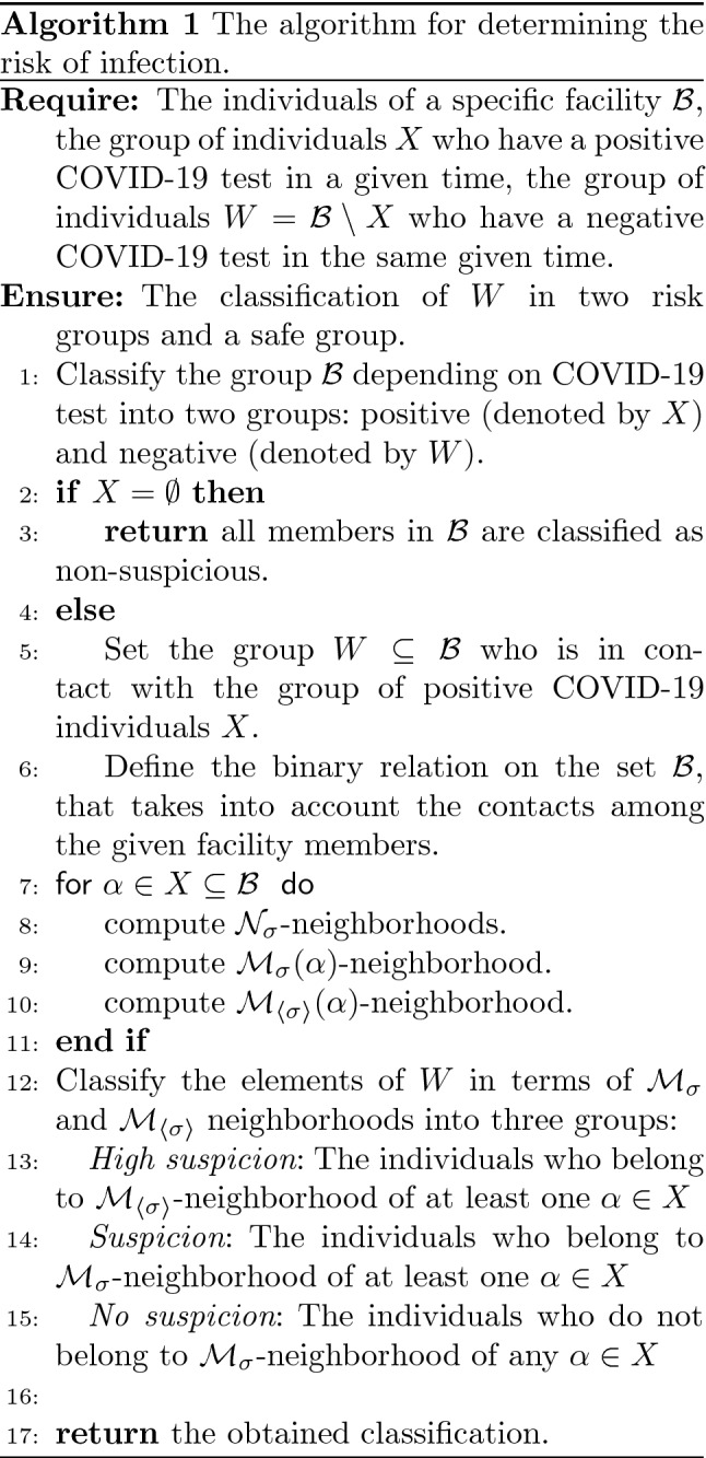

Discussions: strengths and limitations

• Strengths

  1. Determination of the smallest and largest ${\mathcal{M}}_{\sigma }$-neighborhoods from all $\sigma$ under any arbitrary relation (see, item (iii) of Proposition 6 and Corollary 7). In fact, this is a unique characterization of ${\mathcal{M}}_{\sigma }$-neighborhoods. The previous types of neighborhoods, given in (Abd El-Monsef et al. 2014; Abo-Tabl 2011; Allam et al. 2005, 2006; Al-shami 2021a; Al-shami et al. 2021b; Yao 1996, 1998), do not have this characterization; their determination is limited on the disjoint two sets $\{i,r,l,u\}$ and $\{⟨i⟩,⟨r⟩$, $⟨l⟩,⟨u⟩\}$. This matter leads to compare ${\mathcal{M}}_{\sigma }$-approximations and ${\mathcal{M}}_{⟨\sigma ⟩}$-approximations as investigated in Proposition 23 and to compare ${\mathcal{A}}_{\sigma }$-accuracy and ${\mathcal{M}}_{⟨\sigma ⟩}$-accuracy measures as investigated in Corollary 24. Whereas, we cannot compare between these two types of neighborhoods (approximations, accuracy measures) generated from $({\mathcal{N}}_{\sigma },{\mathcal{N}}_{⟨\sigma ⟩})$, $({\mathcal{E}}_{\sigma },{\mathcal{E}}_{⟨\sigma ⟩})$, and $({\mathcal{C}}_{\sigma },{\mathcal{C}}_{⟨\sigma ⟩})$ under an arbitrary relation. To validate this matter, let $(\mathcal{B},\theta ,{\zeta }_{\sigma })$ be a $\sigma$-NS as given in Example 1. Then ${\mathcal{N}}_r(\delta )={\mathcal{E}}_r(\delta )=\{\gamma \}$ and ${\mathcal{N}}_{⟨r⟩}(\delta )={\mathcal{E}}_{⟨r⟩}(\delta )=\{\beta ,\delta \}$ are incomparable; also, ${\mathcal{C}}_r(\delta )=\{\delta ,\gamma \}$ and ${\mathcal{C}}_{⟨r⟩}(\delta )=\{\alpha ,\beta ,\delta \}$ are incomparable.
  2. Our method keeps the monotonic property for the accuracy and roughness values under any arbitrary relation as illustrated in Proposition 25 and Corollary 26. Whereas, this property is losing or keeping under strict conditions in some foregoing methods. This is due to that our method is depending only on the union of ${\mathcal{N}}_{\sigma }$-neighborhoods which is proportional to the size of the given relations. In contrast, the relations used in the definitions of some methods (i.e.; equality, subset, superset) randomly works with respect to the size of the given relations. To illustrate this matter in case of ${\mathcal{C}}_l$-neighborhoods, let ${\theta }_1=\{(\alpha ,\alpha ),(\alpha ,\beta ),(\beta ,\delta )\}$ and ${\theta }_2={\theta }_1$ $\bigcup \{(\alpha ,\delta ),(\delta ,\alpha )\}$ be two binary relations on $\mathcal{B}=\{\alpha ,\beta ,\delta \}$. Then we have Table 5 below. Taking $V=\{\alpha ,\beta \}$ and $W=\{\beta ,\delta \}$. By calculation, we obtain ${\mathcal{H}}_{1Cl}(V)={\mathcal{H}}_{1Sl}(V)={\mathcal{H}}^{1Cl}(V)={\mathcal{H}}^{1Sl}(V)=V$, ${\mathcal{H}}_{2Cl}(V)=V$, ${\mathcal{H}}_{2Sl}(V)=\{\alpha ,\delta \}$, ${\mathcal{H}}^{2Cl}(V)={\mathcal{H}}^{2Sl}(V)=\mathcal{B}$, ${\mathcal{H}}_{1Cl}(W)={\mathcal{H}}_{1Sl}(W)=\{\delta \}$, ${\mathcal{H}}^{1Cl}(W)={\mathcal{H}}^{1Sl}(W)=\mathcal{B}$, ${\mathcal{H}}_{2Cl}(W)=W$, ${\mathcal{H}}^{2Cl}(W)=\mathcal{B}$, ${\mathcal{H}}_{2Sl}(W)=\{\delta \}$, and ${\mathcal{H}}^{2Sl}(W)=W$. Now, ${\mathcal{A}}_{2Cl}(V)={\mathcal{A}}_{2Sl}(V)=\frac{2}{3}<{\mathcal{A}}_{1Cl}(V)={\mathcal{A}}_{1Sl}(V)=1$, whereas ${\mathcal{A}}_{2Cl}(W)=\frac{2}{3}>{\mathcal{A}}_{1Cl}(W)=\frac{1}{3}$ and ${\mathcal{A}}_{2Sl}(W)=\frac{1}{2}>{\mathcal{A}}_{1Sl}(W)=\frac{1}{3}$.

Table 5.

${\mathcal{N}}_l$-,${\mathcal{C}}_l$- and ${\mathcal{S}}_l$-neighborhoods

	$\alpha$	$\beta$	$\delta$
${\mathcal{N}}_{1l}$	$\{\alpha \}$	$\{\alpha \}$	$\{\beta \}$
${\mathcal{C}}_{1l}$	$\{\alpha ,\beta \}$	$\{\alpha ,\beta \}$	$\{\delta \}$
${\mathcal{S}}_{1l}$	$\{\alpha ,\beta \}$	$\{\alpha ,\beta \}$	$\{\delta \}$
${\mathcal{N}}_{2l}$	$\{\alpha ,\delta \}$	$\{\alpha \}$	$\{\alpha ,\beta \}$
${\mathcal{C}}_{2l}$	$\{\alpha ,\beta \}$	$\{\beta \}$	$\{\beta ,\delta \}$
${\mathcal{S}}_{2l}$	$\{\alpha \}$	$\mathcal{B}$	$\{\beta \}$

• 3.The ${\mathcal{M}}_{\sigma }$-lower and ${\mathcal{M}}_{\sigma }$-upper approximations keep most Pawlak’s properties as we investigated in Proposition 15, Corollary 16, Proposition 17 and Corollary 18. Also, the properties of Pawlak which are losing by ${\mathcal{M}}_{\sigma }$-approximations are preserved under a reflexive condition.
• 4.Our method produces approximations and accuracy values better than the methods given in (Dai et al. 2018) in cases of $\sigma \in \{i,⟨i⟩,⟨r⟩\}$. Also, the approximations and accuracy values generated by our methods are equal to those generated by ${\mathcal{E}}_{\sigma }$-neighborhoods under a symmetric relation for $\sigma \in \{i,r,l,u\}$ (see, item (ii) of Corollary 10).

• Limitations

  1. The approximations and accuracy measures generated from the methods of ${\mathcal{N}}_{\sigma }$-neighborhoods and ${\mathcal{C}}_{\sigma }$-neighborhoods (Al-shami 2021a) are better than our method under a reflexive relation.
  2. Dai et al.’s method (Dai et al. 2018) produces approximations and accuracy values better than our method in case of $\sigma =u$.

Conclusion and future work

One of the considerable approaches to address the issues of vagueness and uncertain knowledge is rough set theory. In this article, we have established novel kinds of neighborhood systems namely ${\mathcal{M}}_{\sigma }$-neighborhoods. We have deliberated some properties concomitant with ${\mathcal{M}}_{\sigma }$-neighborhoods and elucidated their relationships with some neighborhoods types introduced in the literature. Then, we have exploited them to introduce some types of lower and upper approximations. We have compared between them and showed that an ${\mathcal{M}}_{⟨i⟩}$-neighborhood produces the best approximations and highest accuracy measure. Also, we have demonstrated that ${\mathcal{M}}_{\sigma }$-accuracy and ${\mathcal{M}}_{\sigma }$-roughness values are monotonic under any arbitrary relation, where $\sigma \in \{r,l,i,u\}$.

Moreover, we have compared the followed technique with its counterparts induced from the method given in (Dai et al. 2018) in terms of approximations and accuracy measures of subsets. Also, we have proved the identity between our technique and those given in (Amer et al. 2017) under a symmetric relation. Finally, we applied our approach to protect people from infection with the corona-virus COVID-19.

Possible forthcoming works are

• Benefit from ${\mathcal{M}}_{\sigma }$-neighborhoods to generate different topologies which are applied to establish new approximations similar to those given in (Abo-Tabl 2013; Dai et al. 2018; Sun et al. 2019);

• Explore ${\mathcal{M}}_{\sigma }$-neighborhoods system in the areas of soft rough set and fuzzy rough sets.

Funding

This research received no external funding.

Availability of data and material

No data were used to support this study.

Declaration

Conflict of interest

The author declares that there is no conflict of interests regarding the publication of this article.

References

- Abd El-Monsef ME, Embaby OA, El-Bably MK. Comparison between rough set approximations based on different topologies. Int J Granul Comput Rough Sets Intell Syst. 2014;3(4):292–305. [Google Scholar]
- Abo-Tabl EA. A comparison of two kinds of definitions of rough approximations based on a similarity relation. Inf Sci. 2011;181:2587–2596. doi: 10.1016/j.ins.2011.01.007. [DOI] [Google Scholar]
- Abo-Tabl EA. Rough sets and topological spaces based on similarity. Int J Mach Learn Cybern. 2013;4:451–458. doi: 10.1007/s13042-012-0107-7. [DOI] [Google Scholar]
- Abu-Donia HM. Comparison between different kinds of approximations by using a family of binary relations. Knowl-Based Syst. 2008;21:911–919. doi: 10.1016/j.knosys.2008.03.046. [DOI] [Google Scholar]
- Al-shami TM. An improvement of rough sets’ accuracy measure using containment neighborhoods with a medical application. Inf Sci. 2021;569:110–124. doi: 10.1016/j.ins.2021.04.016. [DOI] [Google Scholar]
- Al-shami TM. Improvement of the approximations and accuracy measure of a rough set using somewhere dense sets. Soft Comput. 2021;25(23):14449–14460. doi: 10.1007/s00500-021-06358-0. [DOI] [Google Scholar]
- Al-shami TM, Ciucci D (2022) Subset neighborhood rough sets. Knowl Based Syst 237
- Al-shami TM, Alshammari I, El-Shafei ME. A comparison of two types of rough approximations based on -neighborhoods. J Intell Fuzzy Syst. 2021;41(1):1393–1406. doi: 10.3233/JIFS-210272. [DOI] [Google Scholar]
- Al-shami TM, Fu WQ, Abo-Tabl EA. New rough approximations based on -neighborhoods. Complexity. 2021;2021:6. [Google Scholar]
- Allam AA, Bakeir MY, Abo-Tabl EA. International workshop on rough sets, fuzzy sets, data mining, and granular computing. Lecture Notes in Artificial Intelligence. Regina: Springer; 2005. New approach for basic rough set concepts, 2005; pp. 64–73. [Google Scholar]
- Allam AA, Bakeir MY, Abo-Tabl EA. New approach for closure spaces by relations. Acta Math Acad Paedag Nyiregyháziensis. 2006;22:285–304. [Google Scholar]
- Amer WS, Abbas MI, El-Bably MK. On -near concepts in rough sets with some applications. J Intell Fuzzy Syst. 2017;32(1):1089–1099. doi: 10.3233/JIFS-16169. [DOI] [Google Scholar]
- Dai J, Gao S, Zheng G. Generalized rough set models determined by multiple neighborhoods generated from a similarity relation. Soft Comput. 2018;22:2081–2094. doi: 10.1007/s00500-017-2672-x. [DOI] [Google Scholar]
- El-Bably MK, Al-shami TM (2021) Different kinds of generalized rough sets based on neighborhoods with a medical application. Int J Biomath 14(8)
- Lashin EF, Kozae AM, AboKhadra AA, Medhat T. Rough set theory for topological spaces. Int J Approx Reason. 2005;40:35–43. doi: 10.1016/j.ijar.2004.11.007. [DOI] [Google Scholar]
- Mareay R. Generalized rough sets based on neighborhood systems and topological spaces. J Egypt Math Soc. 2016;24:603–608. doi: 10.1016/j.joems.2016.02.002. [DOI] [Google Scholar]
- Pawlak Z. Rough sets. Int J Inf Comput Sci. 1982;11(5):341–356. doi: 10.1007/BF01001956. [DOI] [Google Scholar]
- Pawlak Z. Rough sets, theoretical aspects of reasoning about data. Dordrecht: Kluwer Academic Publishers; 1991. [Google Scholar]
- Salama AS. Sequences of topological near open and near closed sets with rough applications. Filomat. 2020;34(1):51–58. doi: 10.2298/FIL2001051S. [DOI] [Google Scholar]
- Singh PK, Tiwari S. Topological structures in rough set theory: a survey. Hacettepe J Math Stat. 2020;49(4):1270–1294. [Google Scholar]
- Sun S, Li L, Hu K. A new approach to rough set based on remote neighborhood systems. Math Probl Eng. 2019;2019:8. [Google Scholar]
- Yao YY. Two views of the theory of rough sets in finite universes. Int J Approx Reason. 1996;15:291–317. doi: 10.1016/S0888-613X(96)00071-0. [DOI] [Google Scholar]
- Yao YY. Relational interpretations of neighborhood operators and rough set approximation operators. Inf Sci. 1998;111:239–259. doi: 10.1016/S0020-0255(98)10006-3. [DOI] [Google Scholar]
Associated Data
This section collects any data citations, data availability statements, or supplementary materials included in this article.
Data Availability Statement