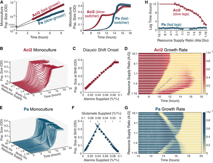
Figure 2. Monoculture growth dynamics reveal Aci2 is a fast‐grower but slow‐switcher whereas Pa is a slow‐grower but fast‐switcher.

- Aci2 and Pa were both grown in monoculture in the two‐resource environment. The same data is shown in both plots. The left plot shows the average of eight technical replicates on a log scale, while the right plot shows each of the replicates on a linear scale. Overlain on the left plot are growth rate fits of g Aci2 = 0.88/h and g Pa = 0.67/h.
- Aci2 was grown with alanine and glutamate supplied at 25 different ratios from 1:16 to 16:1 with the total supply kept constant at 0.1% w/v (Materials and Methods).
- The population size at which Aci2’s diauxic shift occurred is linearly correlated to the alanine supply, indicating that Aci2 initially consumes almost entirely alanine.
- Instantaneous growth rates were extracted from the Aci2 monoculture data (Materials and Methods). A variation in Aci2’s lag time is clearly visible in this representation. An alternative visualization in Appendix S6 plots growth rate on a z‐axis to provide a better visualization of the shape of the growth rate recoveries as functions of time.
- The same monoculture experiments were performed for Pa. The appearance of Pa having a long initial lag is primarily due to the growth that it needs to accomplish before its population size becomes significant on a linear scale as well as a small optical density artifact (Appendix Fig S5).
- Pa’s population size at the onset of its diauxic shift correlates to the supply concentration of whichever resource is supplied in a more limiting amount, indicating coutilization.
- Instantaneous growth rates extracted from the Pa monoculture data.
- Diauxic lag times were fit from the monoculture data (Materials and Methods) and are plotted as circles. Lag times could not be fit for conditions with too little growth on the remaining glutamate. The lag times used in the modeling are shown as lines through the data.
Data Information: More detail on the Pa growth rate fit is provided in Fig EV1C. Data in A were collected at 400 nm. Data in B–G were collected at 600 nm. Example lag time fits are shown in Fig EV2A, and the full set in Appendix Figs S3 and S4.
Source data are available online for this figure.
