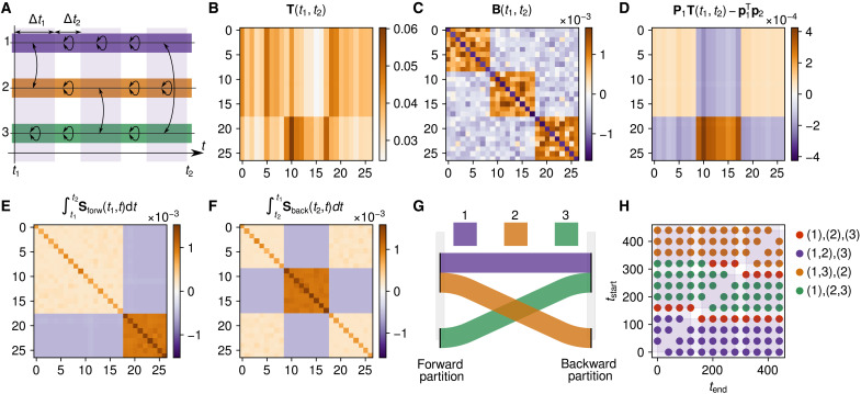
Fig. 2. Flow clustering of a synthetic network with asymmetric temporal paths.

(A) Representation of the different phases of interactions between the three groups of nodes. (B) RW transition matrix computed between the start, t₁, and the end of the three phases, t₂. (C) Modularity matrix computed on the aggregated network ($\mathbf{B}\mathit{=}\mathbf{A}-\frac{{\mathbf{k}}^{\mathit{T}}\mathbf{k}}{\mathbf{2}\mathit{m}}$, where A is the aggregated adjacency matrix, k=A1, and 2m = ∑_ik_i). (D) Covariance matrix, S(t₁, t₂), of the RW process defined in Eq. 12. (E) Integral of the forward process covariance matrix (Eq. 2). (F) Integral of the backward process covariance matrix (Eq. 3). (G) Representation of the forward and backward process in an alluvial diagram. (H) Best partitions found when varying the starting and ending times of the considered interval.