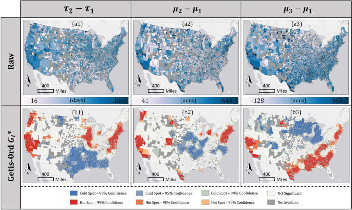
FIGURE 7.

U.S. county‐level spatial patterns of (a1) ${\tau }_2‐{\tau }_1$, (a2) ${\mu }_2‐{\mu }_1$, (a3) ${\mu }_3‐{\mu }_1$ and identified statistically significant hot/coldspots of (b1) ${\tau }_2‐{\tau }_1$, (b2) ${\mu }_2‐{\mu }_1$, (b3) ${\mu }_3‐{\mu }_1$. The calculation procedure of Geitis–Ord $G_i$ is detailed in Appendix C. The Z‐score distribution of $G_i$ is summarized at three significant levels: $\alpha =0.01$ (99% confidence level), $\alpha =0.05$ (95% confidence level), and $\alpha =0.1$ (90% confidence level). Note that (a1), (a2), and (a3) are mapped with 10 classes categorized by Jenks natural breaks (Jenks, 1967)