Figure - PMC

Skip to main content

An official website of the United States government

Here's how you know

Here's how you know

Official websites use .gov
A .gov website belongs to an official government organization in the United States.

Secure .gov websites use HTTPS
A lock ( ) or https:// means you've safely connected to the .gov website. Share sensitive information only on official, secure websites.

View full-text article in PMC

. 2022 Apr 20;4(3):fcac101. doi: 10.1093/braincomms/fcac101

Search in PMC
Search in PubMed
View in NLM Catalog
Add to search

© The Author(s) 2022. Published by Oxford University Press on behalf of the Guarantors of Brain.

This is an Open Access article distributed under the terms of the Creative Commons Attribution License (https://creativecommons.org/licenses/by/4.0/), which permits unrestricted reuse, distribution, and reproduction in any medium, provided the original work is properly cited.

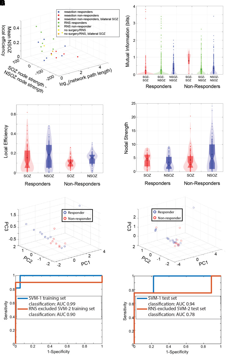
PMC Copyright notice

Graph theoretical measures of the fast ripple MI networks improve the discrimination of non-responders. (A) 3D scatter plot of the FR (>350 Hz) MI global graph theoretical measures (three univariate Wilcoxon rank-sum tests, P > 0.05). (B) Violin plot of MI computed for SOZ–SOZ edges (red), SOZ–NSOZ edges (green), NSOZ–NSOZ edges (blue) across all the responder and non-responder patients (GLMM, P > 0.05). (C) Local efficiency of SOZ (red) and NSOZ (blue) nodes across responder and non-responder patients (GLMM, P > 0.05). (D) Nodal strength of SOZ (red) and NSOZ (blue) nodes across responder and non-responder patients. The location of the node within the SOZ significantly influenced nodal strength (GLMM, P < 0.05), (E, F) 3D scatter plots of the PC scores derived from PCA of the three global measures (A) from all the patients in the training set (E) and combined exploratory and test set (F). The PC2 score was significantly different in the responders compared with non-responders for the training set (rank-sum, P = 0.03) and the combined exploratory and test set patients (rank-sum, P = 0.01). However, only in the latter group did the effect survive after Bonferroni–Holm correction. The PC1 and PC3 scores were not significantly different rank-sum, P > 0.05). (G, H, blue) The ROC curve for non-responder classification in the exploratory dataset (G, n = 19 responders, n = 11 non-responders/no resection or RNS) and in the test dataset (H, n = 9 responders, 4 non-responders/no resection or RNS) by the SVM-1 trained using the SOZ, and FR (>350 Hz) distance, rate–distance and three MI global metric predictors derived from all the exploratory dataset patients. (G, H, red) The ROC curve for non-responder classification using SVM-2 in the exploratory (n = 12 responders, n = 10 non-responders/no resection or RNS) and test set patients (H, n = 9 responders, 4 non-responders/no resection or RNS). SVM-2 excluded RNS implant only patients in the exploratory dataset prior to training and testing. AUC: area under the ROC curve.