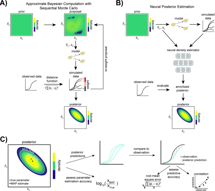
Fig 2. Inference methods and performance assessment.

(A) When using ABC-SMC, in the first iteration, a proposal for the parameters δ_C (GAP1 CNV formation rate) and s_C (GAP1 CNV selection coefficient) is sampled from the prior distribution. Simulated data are generated using either a WF or chemostat model and the current parameter proposal. The distance between the simulated data and the observed data is computed, and the proposed parameters are weighted by this distance. These weighted parameters are used to sample the proposed parameters in the next iteration. Over many iterations, the weighted parameter proposals provide an increasingly better approximation of the posterior distribution of δ_C and s_C (adapted from [68]). (B) In NPE, simulated data are generated using parameters sampled from the prior distribution. From the simulated data and parameters, a density-estimating neural network learns the joint density of the model parameters and simulated data (the “amortized posterior”). The network then evaluates the conditional density of model parameters given the observed data, thus providing an approximation of the posterior distribution of δ_C and s_C (adapted from [50,68].) (C) Assessment of inference performance. The 50% and 95% HDRs are shown on the joint posterior distribution with the true parameters and the MAP parameter estimates. We compare the true parameters to the estimates by their log ratio. We also generate posterior predictions (sampling 50 parameters from the joint posterior distribution and using them to simulate frequency trajectories, ⍴_i), which we compare to the observation, o_i, using the RMSE and the correlation coefficient. ABC-SMC, Approximate Bayesian Computation with Sequential Monte Carlo; CNV, copy number variant; HDR, highest density region; MAP, maximum a posteriori; NPE, Neural Posterior Estimation; RMSE, root mean square error; WF, Wright–Fisher.