. 2022 May 11;11:e73346. doi: 10.7554/eLife.73346

Figure 2. Genetic affinities within the genus Equus.

The Honghe (HH), Muzhuzhuliang (MZ), and Shatangbeiyuan (BY) specimens are shown in red, while Asian asses, African asses, zebras, and horses are shown in purple, blue, green, and black, respectively. (A) Principal component analysis (PCA) based on genotype likelihoods, including horses and all other extant non-caballine lineages (16,293,825 bp, excluding transitions). Only specimens whose genomes were sequenced at least to 1.0× average depth of coverage are included. (B) Maximum likelihood tree based on six mitochondrial partitions (representing a total of 16,591 bp). Those E. ovodovi sequences that were previously published are shown in red. The tree was rooted using Hippidion saldiasi and Haringtonhippus francisci as outgroups. Node supports were estimated from 1000 bootstrap pseudo-replicates and are displayed only if greater than 50%. The black line indicates the mitochondrial clades A and B. (C) Maximum likelihood tree based on sequences of 19,650 protein-coding genes, considering specimens sequenced at least at a 3.0× average depth of coverage (representing 32,756,854 bp).

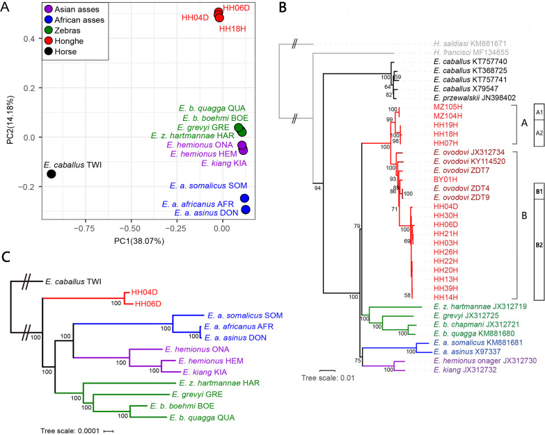
Figure 2.

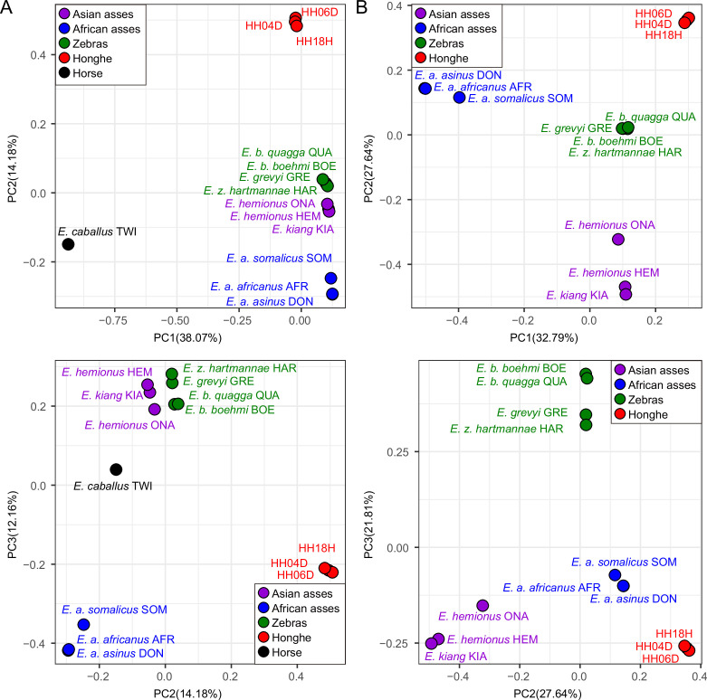
Figure 2—figure supplement 1. Principal component analysis (PCA) based on genotype likelihoods using the horse reference genome.

Figure 2—figure supplement 1.

(A) Including and (B) excluding the outgroup individual underlying the horse reference genome (TWI) (Kalbfleisch et al., 2018). Sequence data were aligned against the horse reference genome (Kalbfleisch et al., 2018).
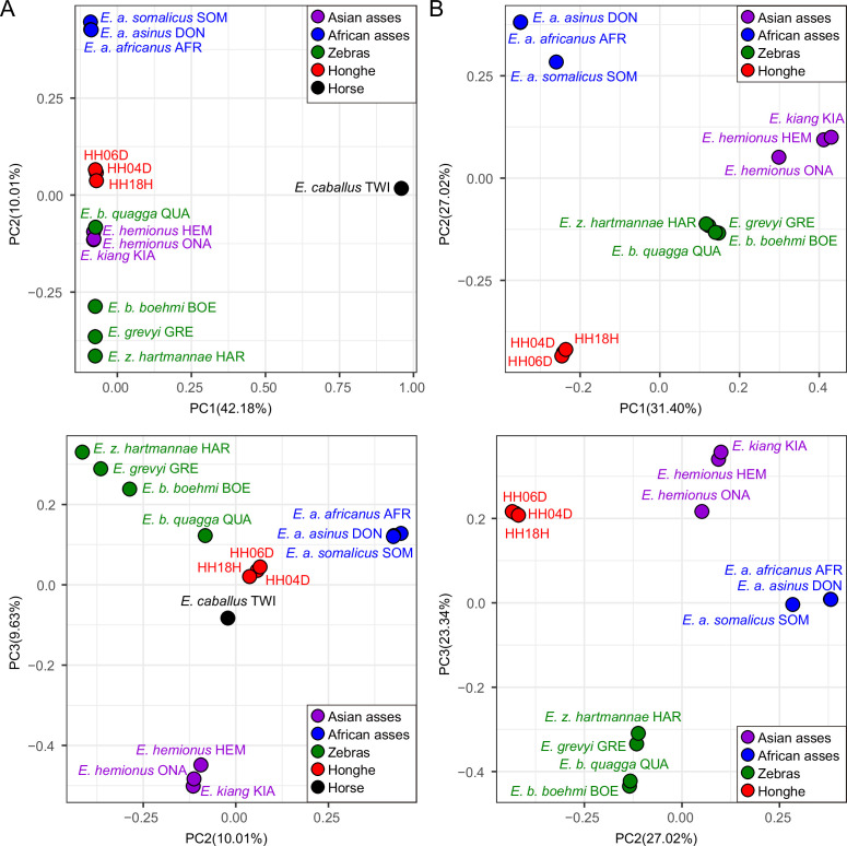
Figure 2—figure supplement 2. Principal component analysis (PCA) based on genotype likelihoods using the donkey reference genome.

Figure 2—figure supplement 2.

(A) Including and (B) excluding the outgroup individual underlying the horse reference genome (TWI) (Kalbfleisch et al., 2018). Sequence data were aligned against the donkey reference genome (Renaud et al., 2018).
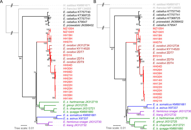
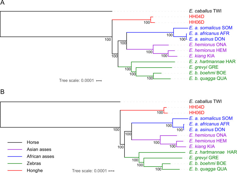
Figure 2—figure supplement 3. RAxML-NG (GTR+GAMMA model) maximum likelihood phylogeny of complete mitochondrial sequence data.

Figure 2—figure supplement 3.

(A) Including the control region. (B) Excluding the control region. Node support was estimated from 1000 bootstrap pseudo-replicates and the tree was manually rooted using Hippidion saldiasi.
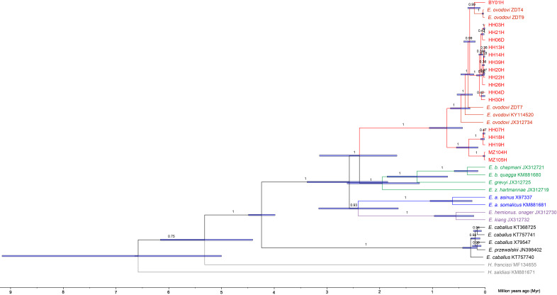
Figure 2—figure supplement 4. Bayesian mitochondrial phylogeny based on six partitions and using Hippidion saldiasi as outgroup.

Figure 2—figure supplement 4.

The tree was reconstructed using a total number of 1000 million Markov Chain Monte Carlo (MCMC) states in BEAST (sampling frequency = 1 every 10,000, burn-in = 25%). The substitution models applied to the six sequence partitions were the TrN+I+G model (first codon position = 3802 sites), the TrN+I model (second codon position = 3799 sites), the GTR+I+G model (third codon position = 3799 sites), the HKY+I model (transfer RNAs = 1517 sites), the TrN+I+G model (ribosomal RNAs = 2556 sites), and the HKY+I+G model (control region = 1192 sites).
Figure 2—figure supplement 5. Exome-based maximum likelihood phylogeny rooted by the horse lineage.

Figure 2—figure supplement 5.

(A) Using sequence alignments against the horse reference genome (Kalbfleisch et al., 2018). (B) Using sequence alignments against the donkey reference genome (Renaud et al., 2018). Node supports were estimated from 100 bootstrap pseudo-replicates.
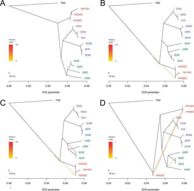
Figure 2—figure supplement 6. TreeMix analysis based on transversions and using the horse reference genome.

Figure 2—figure supplement 6.

Sequence data were mapped against the horse reference genome (Kalbfleisch et al., 2018). A total of 0–3 migration edges were considered. The result of each analysis is shown in panels (A) – (D), respectively. Considering additional migration edges did not improve the variance explained by the TreeMix model (Supplementary file 1f).
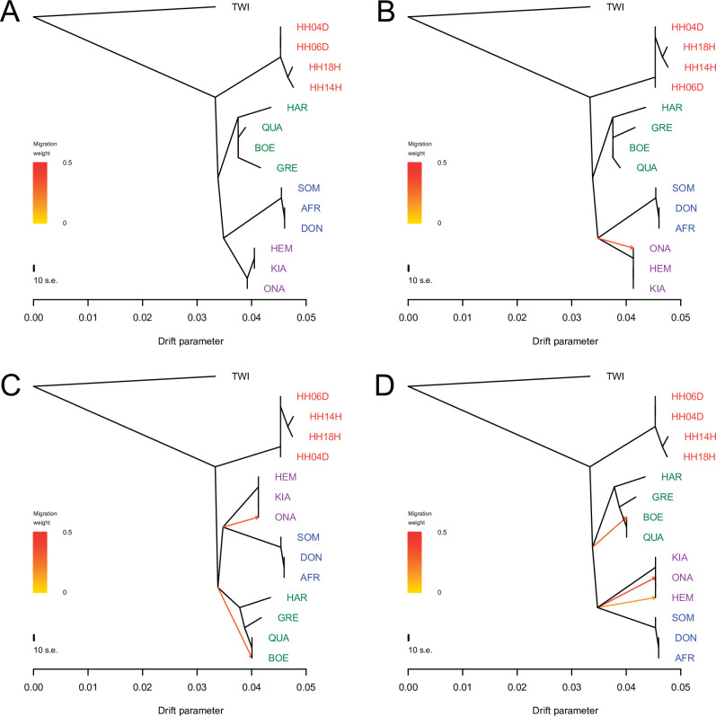
Figure 2—figure supplement 7. TreeMix analysis based on transversions and using the donkey reference genome.

Figure 2—figure supplement 7.

Sequence data were mapped against the donkey reference genome (Renaud et al., 2018). A total of 0–3 migration edges were considered. The result of each analysis is shown in panels (A) – (D), respectively. Considering additional migration edges did not improve the variance explained by the TreeMix model (Supplementary file 1f).
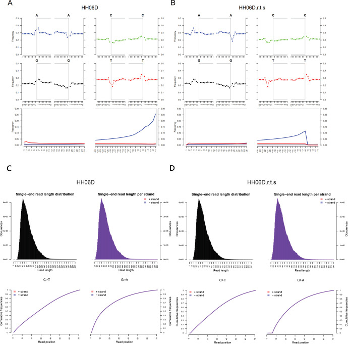
Figure 2—figure supplement 8. DNA damage patterns and the mapped read length distribution plots from mapDamage2 for HH06D.

Figure 2—figure supplement 8.

(A, C) Before rescaling and trimming and (B, D) after rescaling and trimming the region comprising the five first and last nucleotides sequenced.
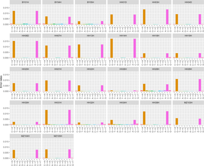
Figure 2—figure supplement 9. Error profiles of the 26 ancient genomes characterized in this study.

Figure 2—figure supplement 9.

After trimming and rescaling, reads showing mapping quality scores inferior to 25 and bases showing quality scores inferior to 20 were disregarded.