A simulation study on the statistical monitoring of condemnation rates from slaughterhouses for syndromic surveillance: an evaluation based on Swiss data

SUMMARY

Syndromic surveillance (SyS) systems currently exploit various sources of health-related data, most of which are collected for purposes other than surveillance (e.g. economic). Several European SyS systems use data collected during meat inspection for syndromic surveillance of animal health, as some diseases may be more easily detected post-mortem than at their point of origin or during the ante-mortem inspection upon arrival at the slaughterhouse. In this paper we use simulation to evaluate the performance of a quasi-Poisson regression (also known as an improved Farrington) algorithm for the detection of disease outbreaks during post-mortem inspection of slaughtered animals. When parameterizing the algorithm based on the retrospective analyses of 6 years of historic data, the probability of detection was satisfactory for large (range 83–445 cases) outbreaks but poor for small (range 20–177 cases) outbreaks. Varying the amount of historical data used to fit the algorithm can help increasing the probability of detection for small outbreaks. However, while the use of a 0·975 quantile generated a low false-positive rate, in most cases, more than 50% of outbreak cases had already occurred at the time of detection. High variance observed in the whole carcass condemnations time-series, and lack of flexibility in terms of the temporal distribution of simulated outbreaks resulting from low reporting frequency (monthly), constitute major challenges for early detection of outbreaks in the livestock population based on meat inspection data. Reporting frequency should be increased in the future to improve timeliness of the SyS system while increased sensitivity may be achieved by integrating meat inspection data into a multivariate system simultaneously evaluating multiple sources of data on livestock health.

INTRODUCTION

Health surveillance is the ongoing, systematic collection, analysis, interpretation and dissemination of data regarding health-related events. Surveillance is critical for an effective early response (to reduce morbidity and mortality) upon the emergence of health problems; and is used to identify changes in the nature or extent of health problems and the effectiveness of actions to improve health [1]. At the beginning of the 21st century, the development of a new type of passive surveillance system, called syndromic surveillance (SyS), highlighted the potential offered by the automated tracking of disease indicators which may signal the onset of epidemics [2].Veterinary SyS is not based on laboratory-confirmed diagnosis of a disease, but on non-specific health indicators (e.g. non-slaughter mortality or number of individuals presenting clinical signs) termed ‘syndromes’ [Triple-S definition of syndromic surveillance (http://www.syndromicsurveillance.eu/)]. Thus, SyS systems seek to exploit new and varied sources of health-related data, some of which may be collected by the animal production industry for purposes other than surveillance (e.g. economic) [3].

Meat inspection data may be suitable for SyS for several reasons. First, it contains large amounts of records routinely collected over several years, providing the possibility to use historical data for constructing a baseline model to define the expected normal behaviour of the indicator monitored. Second, in countries in which the reporting of data is compulsory (e.g. the EU), coverage of the majority of the slaughtered population is ensured and existing reporting channels can be used, thereby reducing the costs required for a surveillance system. While systematic collection and use of meat inspection data for epidemiological surveillance is scarce at the EU level [4], a recent inventory of veterinary SyS initiatives in Europe revealed several monitoring systems that used (e.g. Sweden) or planned to use (e.g. France) meat inspection data from slaughterhouses [5].

System users and decision makers need to have a good understanding of the types of disease agents and outbreak scenarios that are likely to be detected by such surveillance systems. However, the evaluation of the performance of such systems in real surveillance environments remains limited (but see [6]). This constitutes one of the obstacles to the use of meat inspection data for prospective epidemiological surveillance. The most informative evaluation scenario would assess system performance by using data from historical outbreaks of the type the system is intended to detect. This is, unfortunately, rarely possible because for the majority of locations in which systems currently are operating, no such historical data exist and little information is available to enable the interpretation of statistical aberrations retrospectively. Another alternative is to use semi-simulated data for evaluation [7], i.e. real baseline data (usually univariate time-series) are injected with (relatively simple) simulated outbreaks. This is preferable to relying on fully simulated data as it is typically difficult to predict how well simulated data approximate the relevant features of real syndrome counts [8].

The aim of our study was to evaluate, using a mixture of real and simulated data, the performance of a quasi-Poisson regression (also known as the improved Farrington) algorithm [9, 10] for the detection of disease outbreaks during post-mortem inspection of slaughtered animals in Switzerland. Baseline data on whole carcass condemnation (WCC) rates for cattle and pigs were generated based on the characteristics of historical Swiss meat inspection data (dataset described in [11]). As system developers are, by nature, uncertain about the types of outbreaks the surveillance system may come across, we defined feature sets of simulated outbreaks (i.e. of different magnitude and duration) to determine the system's ability to detect an outbreak under varying conditions [7]. The outbreak-detection performance of the system was then measured in terms of its ability to detect a signal (i.e. disease outbreak) against background noise (i.e. normally varying baseline).

METHODS

Condemnation data and outbreak simulation

Meat inspection data were extracted from the ‘Fleischkontrolldatenbank’ (FLEKO database) belonging to the Swiss Federal Food Safety and Veterinary Office (FSVO). The FLEKO holds post-mortem meat inspection data from all hoofed animals slaughtered in Switzerland. Depending on the observations made by the meat inspector (none, generalized vs. localized conditions), the carcass can either be (1) classified as entirely fit for human consumption; (2) partially condemned (only parts of the carcass unfit for human consumption are removed) or (3) wholly condemned (this includes organs and blood). Meat inspectors must report the number of animals slaughtered under normal and emergency (sick or injured) conditions, the number of WCCs, and the reason for condemnation† to the veterinary authorities on a monthly basis. More information on the database can be found in [11]. This study uses data on the number of WCCs of cattle and pigs slaughtered in Switzerland between 1 January 2007 and 31 December 2012 (Table 1). All statistical analyses were performed in R [12] using the ‘surveillance’ package [13]. No major disease outbreaks took place in Swiss cattle or pig populations during this time, so these time-series are assumed to be epidemic free. Both slaughters under normal and emergency conditions were considered.

Table 1.

Number of slaughters and condemnations per animal type and slaughter group between 2007 and 2012

	Number of slaughters	Number of condemnations	%
Cattle	3 750 805	5863	0·16
Cattle (E)	65 304	13 322	20·4
Pigs	16 517 599	25 310	0·15
Pigs (E)	33 720	3288	9·75

E, Slaughtered under emergency conditions.

The four time-series (number of condemned carcasses per month, y_t) were retrospectively modelled following a framework proposed by [14] and implemented in the R function ‘hhh4’. As preliminary analyses using Poisson models showed the presence of overdispersion, the outcome y_t was assumed to follow a negative binomial distribution with mean μ_t. The mean monthly incidence (μ_t) was decomposed additively into an autoregressive component and an endemic component:

The autoregressive component (λ_t) can capture possible outbreaks and can include a seasonal pattern or a long-term trend. The endemic component (ν_t) models the baseline counts and can include seasonality and trend. It is multiplied by the offset (e_t) to adjust for variation in the number of total animals slaughtered per month [15]. The following parametric models for the endemic and autoregressive components were used:

In the endemic part, a baseline condemnation rate is captured with the intercept α, a time trend is captured with the parameter β, and a seasonal component is captured through {S_t}. In the autoregressive component, a baseline estimate of the impact of the observation from the previous month on the current month is estimated with τ. A long-term trend for the dependence of the observations on the previous ones can be estimated with the parameter ω. A seasonal pattern within the autoregressive part can also be estimated through {A_t}.

Four different types of trends were tested for β and ω based on visual inspection of the raw time-series and findings from [11]: no trend (t₀), a (log-)linear trend (t₁), a (log-)linear trend starting in 2010 (t₂₀₁₀), and no trend but a shift in the intercept in 2010 (j₂₀₁₀). Seven different types of seasonality were tested for {S_t} and {A_t}: no seasonality (s₀), a seasonal impact of each month (monthly), an impact of December only (dec) and seasonality with up to |H| = 4 harmonics per year modelled by a combination of sine and cosine functions as in [14] (s₁–s₄). All combinations of the different seasonal patterns and long-term trends within the autoregressive and endemic components were tested for each time-series. Furthermore, models excluding the autoregressive or the endemic component were also evaluated. Model selection (see Supplementary material) was based on Bayesian Information Criterion (BIC) as it does not over-fit the data [16].

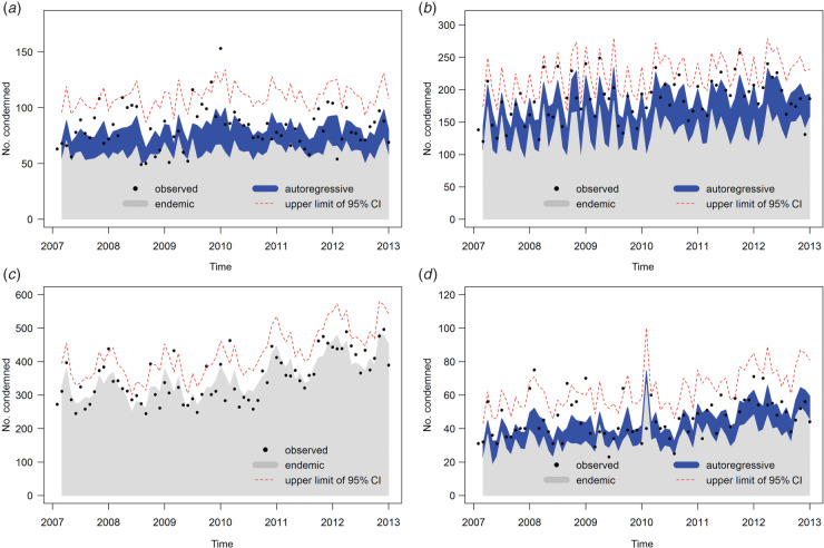
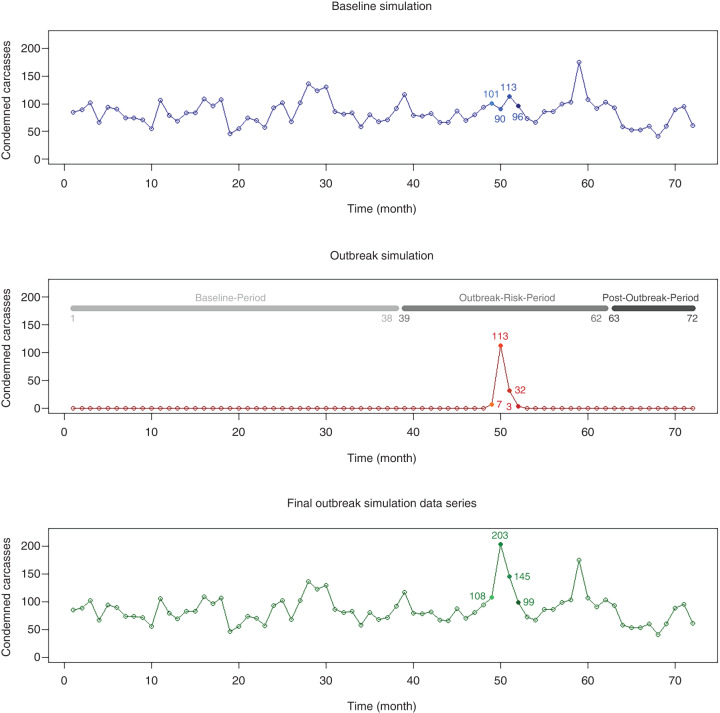
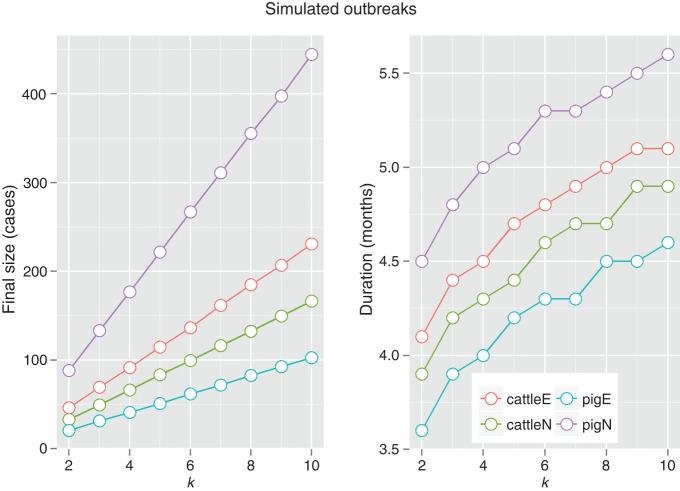
The best retrospective models in terms of BIC (Table 2, Fig. 1) were used to simulate baseline time-series with a length of 72 months. The time-series thus generated were split into three categories: a ‘baseline’ period (38 months), an ‘outbreak-risk’ period (24 months) and a ‘post-outbreak’ period of 10 months (Fig. 2). One outbreak was added to each simulated baseline series, with a random outbreak size and starting point t_i (within the ‘outbreak-risk’ period) as in [10]. Figure 2 helps to visualize the generation process of one simulation. Outbreak sizes were randomly generated as Poisson variables with a mean equal to k times (with k from 2 to 10) the standard deviation of the baseline count at t_i. Preliminary analyses showed that k values >10 produced abnormally large outbreaks which would be, in practice, detected rapidly by the veterinary authorities through other surveillance channels. Outbreak cases were then distributed in time according to a lognormal distribution with mean 0 and standard deviation 0·5. The mean duration of the simulated outbreaks increased with k, but remained in the limited range of 3·6–5·6 months, a realistic duration for disease outbreaks of low mortality which may go unnoticed and uncontrolled by the veterinary authorities for several weeks. The baseline time-series exhibited large variation in standard deviations resulting in more pronounced differences in the final outbreak sizes (Fig. 3). For each parameter k, 1000 time-series were simulated.

Table 2.

Best retrospective (hhh4) models for the four time-series

	Cattle	Cattle (E)	Pigs	Pigs (E)
TrendAR	No	No	AR component excluded	No
TrendEND	No	Log-linear	Log-linear starting in 2010	No
SeasonAR	No	No	AR component excluded	No
SeasonEND	No	No	Sine-cosine 1 harmonic	No

E, Slaughtered under emergency conditions; trendAR, trend in the autoregressive component (λ_t); seasonAR, seasonality in the autoregressive component (λ_t); trendEND, trend in the endemic component (ν_t); seasonEND, seasonality in the endemic component (ν_t).

Fig. 1.

Best retrospective model fit according to the Bayesian Information Criterion for (a) cattle slaughtered under normal conditions, (b) cattle slaughtered under emergency conditions, (c) pigs slaughtered under normal conditions, and (d) pigs slaughtered under emergency conditions.

Fig. 2.

Illustration of outbreak data simulation and inclusion into the time-series.

Fig. 3.

Mean final outbreak size (number of additional condemnations) and duration (in months) over the 1000 simulations for each parameter k. CattleE, cattle slaughtered under emergency conditions; cattleN, cattle slaughtered under normal conditions; pigE, pigs slaughtered under emergency conditions; pigN, pigs slaughtered under normal conditions.

Prospective analysis

The improved Farrington algorithm [9, 10] was applied for outbreak detection on each simulated time-series using the ‘farringtonFlexible’ function in R. The algorithm fits a log-linear quasi-Poisson model using the available baseline data (historic data). The amount of historic data used can be chosen (with parameters b and w) so that only recent values, within the time window (2w + 1) months from the last b years from the current time point, are included to fit the model:

The model can include a baseline incidence rate α, a trend β, a seasonal pattern f_t and the population offset. The outbreak detection performance of the improved Farrington algorithm was compared for different sets of parameters (Table 3). Parameter set 1 was derived from the insight gained from the retrospective analyses. For example, a trend was only included if there was evidence for a trend based on the retrospective analysis; otherwise no trend was fitted. Seasonality was either excluded or included (based on the retrospective analyses) using the {noPeriods} argument. A number of seasonal periods are modelled by a zero-order spline function with {noPeriods+1} knots.

Table 3.

Different sets of parameters used in the improved Farrington algorithm during prospective outbreak detection

Improved Farrington algorithm*	Cattle	Cattle (E)	Pigs	Pigs (E)
Parameter set 1	b = 2	b = 2	b = 3	b = 2
	w = 6	w = 6	w = 2	w = 6
	trend = FALSE	trend = TRUE	trend = TRUE	trend = FALSE
	noPeriods = 1	noPeriods = 1	noPeriods = 1	noPeriods = 1
Parameter set 2	b = 3	b = 3	b = 3	b = 3
	w = 0	w = 0	w = 0	w = 0
	trend = FALSE	trend = TRUE	trend = TRUE	trend = FALSE
	noPeriods = 1	noPeriods = 1	noPeriods = 1	noPeriods = 1
Parameter set 3	Set 1 with trend = TRUE	NA	NA	Set 1 with trend = TRUE

E, Slaughtered under emergency conditions.

^*The amount of historic data used to fit the model can be chosen such that only recent values within the time window (2w + 1) months from the last b years from the current time point are included. A number of seasonal periods are modelled by a zero-order spline function with {noPeriods + 1} knots.

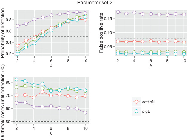
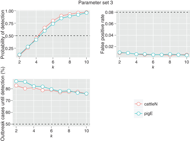
Parameter sets 2 and 3 were chosen to increase the probability of detection (POD) of small outbreaks (defined as 2 < k < 4). We hypothesized that the performance may be improved by varying the amount of historic data used to fit the model (set 2); or by including a trend in the model (set 3) if not previously included (as suggested in [10]). A population offset (total number of animals slaughtered) was used in all models.

The models were then used to derive prospective predictions (and upper confidence limits) for the number of condemnations in a given month. The one-sided confidence limit was derived from the (1 – α)*100% quantile of the normally distributed estimates (α = 0·025 was used). A statistical alarm was raised when an observed value (y₀) at the current time point (t₀) exceeded the confidence limit (U₀) according to the following Z score:

with defined as the expected value at t₀

The following performance criteria were calculated and averaged over 1000 simulations for each parameter k. The false-positive rate (FPR) was defined as the number of statistical alarms during outbreak-free months within the outbreak-risk period divided by the total number of months that were outbreak free within the same period. The POD was obtained by dividing the number of outbreaks that were detected by the total number of simulations tested. An outbreak was detected if there was at least one alarm during the course of the outbreak. Thus the FPR indicates a rate per month and POD a rate per outbreak. The mean time to detection in months (TTD) and the mean percentage of cases until detection (CUD) were calculated only from simulations during which an outbreak was detected.

RESULTS

Prospective outbreak detection

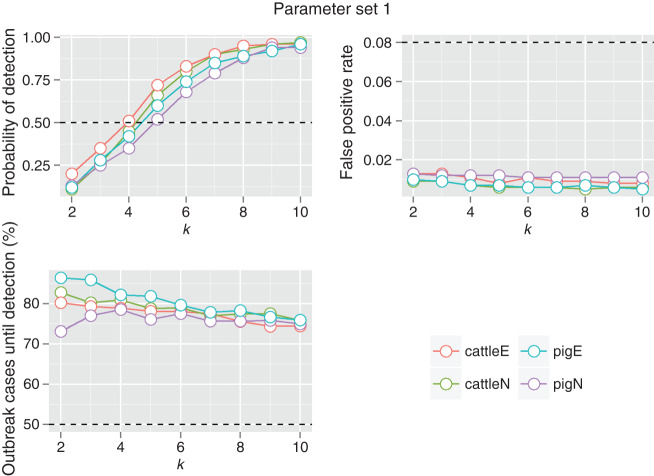
Under parameter set 1 (which was derived from the retrospective analyses), the improved Farrington algorithm detected <50% of small outbreaks (Fig. 4). The number of outbreak-related WCCs had to reach at least 50% (range 49–104%) of the mean monthly baseline counts for the algorithm to detect at least one in every two outbreaks. A satisfactory POD (>80%) was only achieved for the time-series in which large outbreaks (defined as 8 < k < 10) were inserted. When the algorithm correctly identified an outbreak, the statistical alarm was raised, on average, 1 month after the simulated outbreak started (range 0·9–1·1 months), by which time between 73% and 86% of all outbreak cases had already been introduced into the slaughtered population, i.e. the larger part of the epidemic had run its course unmanaged. The FPRs (range 0·005–0·013/month) were satisfactory, leading to one false-positive alarm (and ensuing epidemiological investigation) every 6·4–16·6 years.

Fig. 4.

Outbreak detection performance of the improved Farrington algorithm with parameter set 1. Probability of detection (POD), false-positive rate (FPR) and percentage of cases until detection (CUD) are averaged over 1000 simulations for each parameter k. The dashed line indicates a POD of 0·5, a FPR of 0·08 that corresponds to one false-positive alarm per year, and a CUD of 50% of outbreak cases, respectively. CattleE, cattle slaughtered under emergency conditions; cattleN, cattle slaughtered under normal conditions; pigE, pigs slaughtered under emergency conditions; pigN, pigs slaughtered under normal conditions.

The parameters of the improved Farrington algorithm were then modified (set 2) to try and increase the POD of small outbreaks by varying the amount of historic data used to fit the model (Fig. 5). The POD for the smallest simulated outbreaks (k = 2) increased (range 123–271%); however, a trade-off was apparent with POD of the largest outbreaks (k = 10) being lower (range 2–17%) when more historic data were used to fit the model. The number of outbreak-related WCCs had to reach at least 25% (range 25–111%) of the mean monthly baseline counts for the algorithm to detect at least one in every two outbreaks. Comparing the performance of both parameter sets for the improved Farrington algorithm, we found that parameter set 2 reduced the threshold of outbreak-related WCCs required to reach a POD of 50% for pigs slaughtered under normal conditions (222 and 88 outbreak-related WCCs for sets 1 and 2, respectively). When outbreaks were detected, between 57% and 86% of the outbreak-related WCCs had already gone through meat inspection (range of time to alarm: 0·8–1·3 months). The FPR for pigs slaughtered under normal condition time-series was high (range 0·163–0·173/month), in other words the system would produce a false alarm every 6 months. For the other three time-series, the FPRs were more reasonable, one false alarm every 1·2–16·6 years (range 0·005–0·07/month). Including a trend in the model when not already present (parameter set 3), did nothing to improve the POD or the FPR (Fig. 6).

Fig. 5.

Outbreak detection performance of the improved Farrington algorithm with parameter set 2. Probability of detection (POD), false-positive rate (FPR) and percentage of cases until detection (CUD) are averaged over 1000 simulations for each parameter k. The dashed line indicates a POD of 0·5, a FPR that corresponds to one false-positive alarm per year, and a CUD of 50% of outbreak cases, respectively. CattleE, cattle slaughtered under emergency conditions; cattleN, cattle slaughtered under normal conditions; pigE, pigs slaughtered under emergency conditions; pigN, pigs slaughtered under normal conditions.

Fig. 6.

Outbreak detection performance of the improved Farrington algorithm with parameter set 3. Probability of detection (POD), false-positive rate (FPR) and percentage of cases until detection (CUD) are averaged over 1000 simulations for each parameter k. The dashed line indicates a POD of 0·5, a FPR that corresponds to one false-positive alarm per year, and a CUD of 50% of outbreak cases, respectively. CattleN, cattle slaughtered under normal conditions; pigE, pigs slaughtered under emergency conditions.

DISCUSSION

The choice of model parameters had an impact on the ability of the improved Farrington algorithm to detect simulated outbreaks in the WCC surveillance data collected in Switzerland. When using parameters based on the retrospective analyses of 6 years of historic data (set 1), the algorithm performed reasonably well (in terms of POD) for the detection of large outbreaks but performed poorly in detecting smaller outbreaks. One explanation could be the high variation in the baseline counts and the low amount of data used for parameter estimation. The former results in high estimates of mean incidence rates, while the latter leads to estimates with high standard errors. Both contribute to increased detection thresholds, making it difficult to detect outbreaks with a low number of cases. The POD of smaller outbreaks was better after decreasing the time window (w) and increasing the amount of years (b) used to fit the model (parameter set 2) although this reduced the POD for larger outbreaks. Noufaily et al. suggested including a trend in the model to improve POD [10] (parameter set 3) but we found no difference between the performance indicators of the algorithm when parameterized with set 1 or set 3.

The use of a 0·975 quantile generated a low FPR in most of the series tested. A statistical alarm generated by the system would result in the initiation of a response protocol by the relevant authorities. The first step in investigating an alarm is confirmation of the signal. The individual cases that triggered the alarm must be examined to obtain geographical (and potentially demographic) data. Then, if the signal does not appear to be the result of duplication of individual case data or data entry error, the specificity of the signal must be increased (e.g. by a phone call to the meat inspectors at the reporting sites, by dispatching a team of epidemiologists in the field, etc.). The cost linked to a statistical alarm investigation (time and people resources) in our system would be acceptable for a FPR of 0·08 or lower (⩽1 false alarm per year). This was the case for all series screened with the first parameter set and most series screened with the second parameter set. Applying parameter set 2 to the time-series of pigs slaughtered under normal conditions resulted in an average false alarm rate of 1 every 6 months, a FPR that would probably be too costly for the system's users.

High variation in the baseline counts constitutes one of major limitations of the use of the Swiss WCC data for early outbreak detection. The POD for smaller outbreaks may be increased by minimizing the variance of the WCC time-series. One possibility could be to apply such algorithms to the time-series of some specified reason for WCC. Abscesses and acute lesions are the most commonly reported reason for WCC for Swiss pigs and cattle, respectively [11]. While sub-setting the WCC time-series may slightly reduce the variance observed on a monthly level, the SyS system should be monitoring more than one WCC reason as these are non-specific health indicators and the system should be able to detect any outbreak caused by unspecified or unknown pathogens. The next step should be to monitor concomitantly several time-series (corresponding to different reasons for WCCs in pigs slaughtered under normal conditions, for example) using multivariate methods (e.g. [17, 18]). We could also stratify the WCC data by age, sex and production type in an attempt to reduce variance; however, such data are not currently recorded by the meat inspectors. We have also shown in a previous study [11] that WCC rates differed between large and small slaughterhouses. However, as long as the proportion of animals going to small vs. large slaughterhouses is constant through time, the effects above may not be important for outbreak detection of the aggregated time-series, but will become relevant during the more detailed investigation of statistical alarms.

Outbreak simulation was performed according to the methods outlined in [10]. Noufaily et al. chose a lognormal distribution to simulate outbreaks in the weekly counts of isolates reported to the Health Protection Agency. Transferring Noufaily's methodology [10] to monthly data may have its limitations. While the outbreaks we simulated were quite long (range 3·6–5·6 months), the majority of the outbreaks detected were flagged within 1 month of their occurrence. Unfortunately, due to the lognormal distribution of the outbreaks, more than 50% of the outbreak cases had already occurred at the time of detection. Different outbreak shapes such as flat, linear or exponential could be simulated using different methods (see [6, 19]). However, the assumed temporal distribution of any simulated outbreak constitutes a challenge to the early detection of outbreaks using monthly surveillance data. The applicability of the developed algorithms should be further evaluated in the future when the reporting frequency of the meat inspection data has increased. Statistical process control methods used on weekly WCC data from one large slaughterhouse in the Manche department, France, have recently shown good outbreak detection performances [6].

A limitation of most existing outbreak simulation approaches, including ours, is that they may create signals with insufficient complexity to evaluate the effectiveness of certain algorithms in the scenarios and data environments for which they were designed [20]. For example, we do not explicitly model the disease agent responsible for the simulated outbreak. Strong assumptions about disease-agent parameters (e.g. time spent in the incubation state) would need to be made to develop such a simulation model. However, the aim of this study was to understand the plausible range of detection-performance results for a non-specified outbreak scenario as we cannot predict the pathogen responsible for the next major zoonotic outbreak in Switzerland. While larger outbreaks in the livestock population may be more readily detected using other animal-health data sources, meat inspection data may prove to be a valuable source of data when trying to detect smaller outbreaks which may span a longer time period. Parameter sets for the improved Farrington algorithm that increase the POD of small outbreaks and lead to <1 investigation per year could therefore be considered reasonable by the Swiss veterinary services. Parameter set 2 should be prospectively applied on all the time-series, except the series for pigs slaughtered under normal conditions for which parameter set 1 is preferred. The lack of sensitivity of the system evaluated is a valuable, if not disappointing, output from this study. It highlights the need for the future SyS system planned by the FSVO to integrate diverse data sources on livestock to help increase the sensitivity and timeliness of its statistical output. One possibility would be to collate additional data, such as information on production levels and market prices in order to help interpret more accurately the patterns observed in the WCC time-series. However, no single data source will capture data from all the individuals involved in an outbreak. Some diseases will cause a wide variety of clinical symptoms in different animals and/or will affect different strata of the population. As such, SyS systems should be multivariate by nature, i.e. simultaneously evaluating various combinations of multiple datasets. In the next stage, we will consider integrating the meat inspection data into a multivariate SyS system for production animals in Switzerland, an option that may appeal to decision makers as providing consistent evidence which may be used to suggest inferential accuracy.

DECLARATION OF INTEREST

None.

REFERENCES

- 1.Buehler JW. Surveillance. In: Rothman KJ, Lash TL, Greenland S, eds. Modern Epidemiology, 3rd edn. Philadelphia PA: Lippencott-Raven, 2008, pp. 459–480. [Google Scholar]
- 2.Reingold A. If syndromic surveillance is the answer, what is the question? Biosecurity and Bioterrorism: Biodefense Strategy, Practice, and Science 2003; 1: 77–81. [DOI] [PubMed] [Google Scholar]
- 3.Pavlin JA. Syndromic surveillance for infectious diseases. In: M'ikanatha NM, Lynfield R, Van Beneden CA, de Valk H, eds. Infectious Disease Surveillance. Oxford, UK: John Wiley & Sons Ltd, 2013. [Google Scholar]
- 4.Harley S, et al. Good animal welfare makes economic sense: potential of pig abattoir meat inspection as a welfare surveillance tool. Irish Veterinary Journal 2012; 65: 11. [DOI] [PMC free article] [PubMed] [Google Scholar]
- 5.Dupuy C, et al. Inventory of veterinary syndromic surveillance initiatives in Europe (Triple-S project): Current situation and perspectives. Preventive Veterinary Medicine 2013; 111: 220–229. [DOI] [PubMed] [Google Scholar]
- 6.Dupuy C, et al. Pilot simulation study using meat inspection data for syndromic surveillance: use of whole carcass condemnation of adult cattle to assess the performance of several algorithms for outbreak detection. Epidemiology and Infection. Published online: 8 January 2015. doi: 10.1017/S0950268814003495. [DOI] [PMC free article] [PubMed] [Google Scholar]
- 7.Mandl K, Reis B, Cassa C. Measuring outbreak-detection performance by using controlled feature set simulations. Morbidity and Mortality Weekly Report 2004; 53 (Suppl.): 130–136. [PubMed] [Google Scholar]
- 8.Jackson ML, et al. A simulation study comparing aberration detection algorithms for syndromic surveillance. BMC Medical Informatics and Decision Making 2007; 7: 6. [DOI] [PMC free article] [PubMed] [Google Scholar]
- 9.Farrington CP, et al. A Statistical algorithm for the early detection of outbreaks of infectious disease. Journal of the Royal Statistical Society 1996; 159: 547–563. [Google Scholar]
- 10.Noufaily A, et al. An improved algorithm for outbreak detection in multiple surveillance systems. Statistics in Medicine 2013; 32: 1206–1222. [DOI] [PubMed] [Google Scholar]
- 11.Vial F, Reist M. Evaluation of Swiss slaughterhouse data for integration in a syndromic surveillance system. BMC Veterinary Research 2014; 10: 33. [DOI] [PMC free article] [PubMed] [Google Scholar]
- 12.R Core Team and R Development Core Team. R: A language and environment for statistical computing. R Foundation for Statistical Computing, Vienna, Austria, 2014.
- 13.Höhle M. surveillance: An R package for the monitoring of infectious diseases. Computational Statistics 2007; 22: 571–582. [Google Scholar]
- 14.Held L, Höhle M, Hofmann M. A statistical framework for the analysis of multivariate infectious disease surveillance counts. Statistical Modelling 2005; 5: 187–199. [Google Scholar]
- 15.Held L, Paul M. Statistical modeling of infectious disease surveillance data. In: M'ikanatha NM, Lynfield R, Van Beneden CA, de Valk H, eds. Infectious Disease Surveillance. Oxford, UK: John Wiley & Sons Ltd, 2013. [Google Scholar]
- 16.Hurvich C, Tsai C-L. Regression and time series model selection in small samples. Biometrika 1989; 76: 297–307. [Google Scholar]
- 17.Banks D, et al. Bayesian CAR models for syndromic surveillance on multiple data streams: theory and practice. Information Fusion 2012; 13: 105–116. [Google Scholar]
- 18.Corberán-Vallet A. Prospective surveillance of multivariate spatial disease data. Statistical Methods in Medical Research 2012; 21: 457–77. [DOI] [PMC free article] [PubMed] [Google Scholar]
- 19.Dórea FC, et al. Syndromic surveillance using veterinary laboratory data: data pre-processing and algorithm performance evaluation. Journal of the Royal Society, Interface 2013; 10: 20130114. [DOI] [PMC free article] [PubMed] [Google Scholar]
- 20.Buckeridge DL, et al. Evaluation of syndromic surveillance systems – design of an epidemic simulation model. Morbidity and Mortality Weekly Report 2004; 53 (Suppl.): 137–143. [PubMed] [Google Scholar]
Associated Data
This section collects any data citations, data availability statements, or supplementary materials included in this article.
Supplementary Materials
For supplementary material accompanying this paper visit https://doi.org/10.1017/S0950268815000989.
click here to view supplementary material